Lomb-Scargle periodograms with astropy: a variable star from irregular nights

The problem: the period of a pulsing star from scattered nights

An RR Lyrae star swells and shrinks with a period of about half a day, and its brightness swings by close to a magnitude in every cycle. The star in this tutorial is modeled on RR Lyr itself, with a period of 0.5668 d. One observer measures it on the clear nights of a four-month season: 60 nights out of 120, one to three exposures a night, each good to 0.05 mag. Daylight cuts a gap into every day, and the weather cuts gaps of several days.

The FFT of The Fourier transform: asking a signal how much of each frequency it contains needs samples on an even grid, and these 122 points have none. The Lomb-Scargle periodogram does not need one. At every trial frequency it fits a sine to the points where they are and records how much of their scatter that sine explains, and the frequency that explains the most is the star's.

Three words from astronomy. Magnitudes run backwards, smaller is brighter, so every light curve below is drawn with the axis flipped and bright at the top. V is the standard green-yellow filter band. RRab is the subclass of RR Lyrae stars that pulse in their fundamental mode, with periods from about 0.3 to 1 d and a light curve like a sawtooth: a fast rise to maximum, then a slow decline.

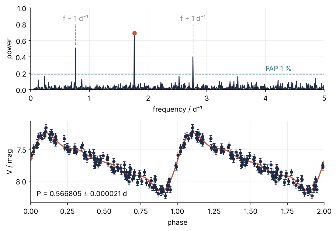
This is where we end up: the periodogram with its highest peak, the two aliases one cycle per day away, and the power a peak must reach to count, above the light curve folded on the period found, with a four-harmonic model through it. The period comes out as 0.566805 ± 0.000021 d, against 0.5668 d put in. Step 6 draws the figure, and each step before it adds one of its parts.

Setup

The star is a Fourier series of four harmonics with the phases of a sawtooth, so it rises fast and fades slowly. The schedule picks the clear nights at random and puts each exposure within 4 h of local midnight. The truth is known only because the data are made.

import numpy as np
import matplotlib.pyplot as plt
from astropy.timeseries import LombScargle

plt.rcParams.update({
    "figure.figsize": (7, 3.6), "figure.dpi": 110,
    "axes.spines.top": False, "axes.spines.right": False,
    "axes.grid": True, "grid.alpha": 0.25,
    "font.size": 11, "lines.linewidth": 1.8,
})
INK, ACCENT, SECOND, MUTED = "#1f2a44", "#c8553d", "#2a7f9e", "#8a8f98"

P_TRUE = 0.5668                             # d, modeled on RR Lyr
V_MEAN = 7.7                                # mag
AMP = np.array([0.32, 0.16, 0.10, 0.06])    # mag, harmonics 1 to 4
SIGMA = 0.05                                # mag, per exposure


def rrlyrae_mag(t):
    """V magnitude at times t in days."""
    k = np.arange(1, 5)[:, None]
    return V_MEAN - (AMP[:, None] * np.sin(2 * np.pi * k * np.asarray(t) / P_TRUE)).sum(axis=0)


def schedule(rng, half_night=4 / 24):
    """Exposure times in days: 60 clear nights of 120, one to three exposures each."""
    nights = np.sort(rng.choice(120, size=60, replace=False))
    per_night = rng.integers(1, 4, size=60)
    # t = 0 is noon before the first night, so midnight falls at n + 0.5
    t = np.repeat(nights, per_night) + 0.5 + rng.uniform(-half_night, half_night, per_night.sum())
    return np.sort(t)


rng = np.random.default_rng(144)
t = schedule(rng)
mag = rrlyrae_mag(t) + rng.normal(0, SIGMA, t.size)
dmag = np.full(t.size, SIGMA)

v_cycle = rrlyrae_mag(np.linspace(0, P_TRUE, 1000))
print(f"{t.size} points on 60 nights over {t[-1] - t[0]:.1f} d, "
      f"model range {v_cycle.max() - v_cycle.min():.2f} mag")

122 points on 60 nights over 117.1 d, model range 0.94 mag

Step 1: Look at the light curve and its gaps

Plot the measurements against time, with the magnitude axis turned upside down, and print the spacing between consecutive points:

fig, ax = plt.subplots(figsize=(7, 3.2))
ax.errorbar(t, mag, dmag, fmt="o", ms=4, capsize=2, lw=1, color=INK)
ax.set(xlabel="t / d", ylabel="V / mag")
ax.invert_yaxis()
plt.show()

gaps = np.diff(t)
print(f"shortest spacing  {gaps.min() * 24 * 60:5.1f} min")
print(f"median spacing    {np.median(gaps) * 24:5.1f} h")
print(f"longest spacing   {gaps.max():5.1f} d")
print(f"distinct spacings {np.unique(gaps).size} of {gaps.size}")

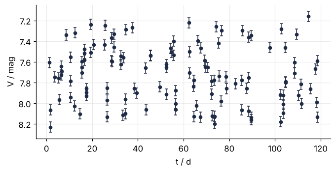
V magnitude against time over 117 days, bright at the top. The points come in clumps one day apart with gaps of several days, and no period is visible.

shortest spacing    2.3 min
median spacing      6.3 h
longest spacing     8.0 d
distinct spacings 121 of 121

Exposures in the same night lie as close as 2.3 min apart, the median spacing is 6.3 h, and the longest gap is 8.0 d. All 121 spacings differ, so there is no grid to put an FFT on. Nothing in the plot gives the period away either: the star moves through most of its range within one night, and the next look comes a day or more later.

Step 2: Compute a periodogram on a grid you choose

LombScargle takes the times, the values, and their uncertainties. At each trial frequency it fits a sine plus a constant to the points by weighted least squares, the fit of Least squares: what a fit minimizes, and why the residuals are squared. The power it reports is the fraction of χ² that the sine removes, χ² being the sum of the squared residuals, each divided by its squared uncertainty. Power 0 means the sine explains nothing beyond the mean, power 1 that it passes through every point. SciPy's scipy.signal.lombscargle does the same fit in angular frequency, but only when you set floating_mean=True and weights, both off by default. Astropy's class adds the false alarm probability and the harmonics used below.

ls = LombScargle(t, mag, dmag)
freq, power = ls.autopower()
print(f"default grid: {freq.size} frequencies up to {freq.max():.2f} 1/d, "
      f"best period {1 / freq[power.argmax()]:.4f} d")

default grid: 1526 frequencies up to 2.61 1/d, best period 0.5666 d

Without arguments, autopower stops at 2.61 d⁻¹. That ceiling is nyquist_factor (5) times N/(2T), an average Nyquist frequency for N points over a span T. It depends on how many points you took, not on how fast the star varies.

The prerequisite's Nyquist frequency is a hard limit because of the equal spacing: above it, a faster sine passes through exactly the same samples as a slower one. With times scattered over the night, two frequencies agree at some samples and not at others, so nothing folds back exactly. The limit comes from the physics instead: RR Lyrae periods lie between 0.2 and 1 d, so search from 0.05 to 5 d⁻¹:

T = t[-1] - t[0]
freq, power = ls.autopower(minimum_frequency=0.05, maximum_frequency=5, samples_per_peak=10)
f_best = freq[power.argmax()]
print(f"{freq.size} frequencies, step {freq[1] - freq[0]:.5f} 1/d, peak width 1/T = {1 / T:.5f} 1/d")
print(f"best: f = {f_best:.4f} 1/d, P = {1 / f_best:.5f} d, power {power.max():.2f}")

fig, ax = plt.subplots(figsize=(7.5, 3.2))
ax.plot(freq, power, color=INK, lw=1.2)
ax.plot(f_best, power.max(), "o", color=ACCENT, ms=6)
ax.annotate(f"P = {1 / f_best:.4f} d", (f_best, power.max()), xytext=(8, -4),
            textcoords="offset points", color=ACCENT)
ax.set(xlabel="frequency / d⁻¹", ylabel="power", xlim=(0, 5), ylim=(0, 1))
plt.show()

5798 frequencies, step 0.00085 1/d, peak width 1/T = 0.00854 1/d
best: f = 1.7645 1/d, P = 0.56673 d, power 0.69

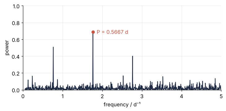
Lomb-Scargle power against frequency from 0.05 to 5 per day. The highest peak, at 1.76 per day or 0.567 d, stands in a forest of lower peaks spaced one per day apart.

The grid step is 1/(T × samples_per_peak), a tenth of the peak width 1/T, so no peak can hide between two grid points. The highest peak sits at 1.7645 d⁻¹, a period of 0.56673 d, with a power of 0.69. It stands in a forest of peaks one cycle per day apart, and the one at 2.76 d⁻¹ lay above the default ceiling.

Step 3: Recognize the one-day aliases

The forest comes from the calendar. The observer can only look at night, so the sampling repeats every day, and the partial agreement of Step 2 becomes nearly complete for f ± 1.

Write the sine at f + 1 as sin(2π(f + 1)t) = sin(2πft + 2πt). Between two exposures exactly one day apart the extra phase 2πt grows by a full turn, so a sine at f + 1, or at f − 1, passes through nearly the same points as the sine at f. Nearly, because the exposures spread over ±4 h around midnight. The clock starts at noon, so midnight falls at half a day, where the extra phase is half a turn, which the fit absorbs into its own phase, and around that offset it scatters by up to ±60°. That is why the aliases are lower than the peak, but not gone.

The window function shows the calendar alone. It is the periodogram of a series of ones at the observed times, with the mean neither subtracted nor fitted, because either would leave nothing to measure:

window = LombScargle(t, np.ones_like(t), fit_mean=False, center_data=False).power(freq)
for c in [1, 2, 3]:
    near = np.abs(freq - c) < 0.05
    print(f"window near {c} 1/d: power {window[near].max():.2f}")

fig, ax = plt.subplots(figsize=(7.5, 2.6))
for c in [1, 2, 3, 4]:
    ax.axvline(c, color=MUTED, ls="--", lw=1)
ax.plot(freq, window, color=SECOND, lw=1.2)
ax.set(xlabel="frequency / d⁻¹", ylabel="window power", xlim=(0, 5), ylim=(0, 1))
plt.show()

window near 1 1/d: power 0.96
window near 2 1/d: power 0.39
window near 3 1/d: power 0.07

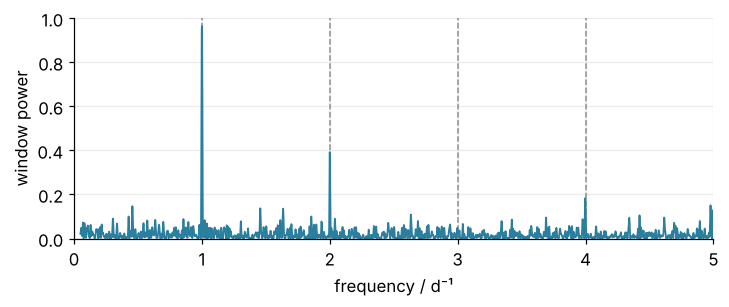
Periodogram of the sampling times alone against frequency. Tall peaks at 1 and 2 per day show that the observing schedule repeats daily.

The window reaches 0.96 near 1 d⁻¹ and 0.39 near 2 d⁻¹. So every peak of the star has copies 1 d⁻¹ to either side:

def local_peak(p, fc, half=0.02):
    """Frequency and power of the highest point of p within half of fc."""
    near = np.abs(freq - fc) < half
    i = np.argmax(p[near])
    return freq[near][i], p[near][i]


for name, fc in [("f - 1", f_best - 1), ("f", f_best), ("f + 1", f_best + 1)]:
    f_peak, p_peak = local_peak(power, fc)
    print(f"{name:5s}  f = {f_peak:.4f} 1/d  P = {1 / f_peak:.4f} d  power {p_peak:.2f}")

f - 1  f = 0.7638 1/d  P = 1.3092 d  power 0.51
f      f = 1.7645 1/d  P = 0.5667 d  power 0.69
f + 1  f = 2.7644 1/d  P = 0.3617 d  power 0.40

The true peak wins here, but a margin of 0.69 against 0.51 is not proof. The test is to fold: compute the phase (t f) mod 1 of every point and plot the magnitude against it. As a number, split the phase into ten bins and take the rms of the points about the mean of their bin, with no model:

def binned_scatter(f, nbins=10):
    """rms of the points about the mean of their phase bin"""
    b = ((t * f) % 1 * nbins).astype(int)
    means = np.array([mag[b == i].mean() for i in range(nbins)])
    return np.sqrt(np.mean((mag - means[b]) ** 2))


f_alias = local_peak(power, f_best - 1)[0]
fig, axes = plt.subplots(2, 1, sharex=True, sharey=True, figsize=(7.5, 4.8))
for ax, f in zip(axes, [f_best, f_alias]):
    ph = (t * f) % 1
    ax.errorbar(np.r_[ph, ph + 1], np.r_[mag, mag], np.r_[dmag, dmag],
                fmt="o", ms=4, capsize=2, lw=1, color=INK)
    ax.text(0.01, 0.05, f"P = {1 / f:.4f} d, binned scatter {binned_scatter(f):.3f} mag",
            transform=ax.transAxes)
    ax.set(ylabel="V / mag")
axes[1].set(xlabel="phase", xlim=(0, 2), ylim=(8.6, 7.0))   # bright at the top, room for the text
plt.show()

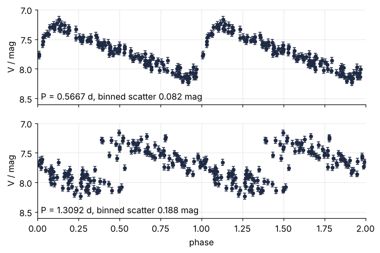
The light curve folded twice, phase 0 to 2. Folded on 0.5667 d the points form a clean sawtooth; folded on the alias at 1.31 d they scatter over the full range.

The binned scatter is 0.082 mag on the peak against 0.188 mag on the alias at 1.31 d. The clean fold sits above the noise of 0.05 mag because the curve changes within a bin, so compare the two folds with each other, not with σ.

Step 4: Judge the peak with a false alarm probability

A power of 0.69 looks high, but high compared with what? The false alarm probability (FAP) is the probability that pure noise at the same times, searched over the same grid, gives a peak at least this high. Pass the limits of the search again, because without them the method assumes the default grid of autopower(). The control uses the same times filled with noise alone:

limits = dict(minimum_frequency=0.05, maximum_frequency=5)
fap = ls.false_alarm_probability(power.max(), **limits)
level = ls.false_alarm_level(0.01, **limits)
print(f"star:  peak power {power.max():.2f}, FAP {fap:.1e}")
print(f"power needed for an FAP of 1 %: {level:.2f}")

noise = rng.normal(V_MEAN, SIGMA, t.size)        # same times, no star
ls_noise = LombScargle(t, noise, dmag)
p_noise = ls_noise.power(freq)
print(f"noise: peak power {p_noise.max():.2f}, "
      f"FAP {ls_noise.false_alarm_probability(p_noise.max(), **limits):.2f}")

star:  peak power 0.69, FAP 5.4e-27
power needed for an FAP of 1 %: 0.19
noise: peak power 0.12, FAP 0.60

The star's peak has an FAP of 5 × 10⁻²⁷. A peak needs a power of 0.19 for an FAP of 1 %, and noise alone reaches 0.12, an FAP of 0.60: this is what nothing looks like. The default method, baluev, gives an upper bound on the FAP (Baluev 2008), but only for a window free of aliases, and this window reaches 0.96 at 1 d⁻¹. At 5 × 10⁻²⁷ that does not change the verdict. Near the 1 % line it can, and method="bootstrap" resamples the data instead, at the price of a periodogram for every resampling.

Step 5: Fit the shape with nterms

The star is not a sine, and a one-term model at the best frequency cannot follow its fast rise. nterms=4 adds sine and cosine pairs at 2f, 3f, and 4f to the same least-squares fit, so its power is still the fraction of χ² removed, now by the bigger model. model(t, f) evaluates the fitted curve at any times:

ls4 = LombScargle(t, mag, dmag, nterms=4)
for name, model in [("1 term ", ls), ("4 terms", ls4)]:
    rms = np.sqrt(np.mean((mag - model.model(t, f_best)) ** 2))
    print(f"{name}: residual rms {rms:.3f} mag")

t_fit = np.linspace(0, 2 / f_best, 400)          # two cycles, phase 0 to 2
ph = (t * f_best) % 1
fig, ax = plt.subplots(figsize=(7.5, 3.2))
ax.errorbar(np.r_[ph, ph + 1], np.r_[mag, mag], np.r_[dmag, dmag],
            fmt="o", ms=4, capsize=2, lw=1, color=INK)
ax.plot(t_fit * f_best, ls.model(t_fit, f_best), color=SECOND, ls="--", lw=1.6)
ax.plot(t_fit * f_best, ls4.model(t_fit, f_best), color=ACCENT)
ax.text(0.30, 7.22, "4 terms", color=ACCENT)
ax.text(0.45, 7.42, "1 term", color=SECOND)
ax.set(xlabel="phase", ylabel="V / mag", xlim=(0, 2))
ax.invert_yaxis()
plt.show()

1 term : residual rms 0.153 mag
4 terms: residual rms 0.058 mag

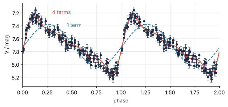
Light curve folded on 0.5667 d with two models. The single sine, dashed, misses the fast rise to maximum; the four-harmonic model follows it.

The residual rms falls from 0.153 mag with one term to 0.058 mag with four, close to the noise of 0.05 mag. The FAP of Step 4 had to be computed with one term: astropy raises NotImplementedError for a multi-term false alarm probability.

Step 6: Pin down the period and its uncertainty

The grid of Step 2 has a step of 0.00085 d⁻¹, which is 24 s in period by δP = P² δf, coarser than the data can pin. Refine on 301 frequencies within ±0.0015 d⁻¹ of the peak, once with one term and once with four:

fine = np.linspace(f_best - 0.0015, f_best + 0.0015, 301)


def refine(y, nterms):
    return fine[LombScargle(t, y, dmag, nterms=nterms).power(fine).argmax()]


f1, f4 = refine(mag, 1), refine(mag, 4)
print(f"grid step in period: Step 2 {(freq[1] - freq[0]) / f_best**2 * 86400:.0f} s, "
      f"fine {(fine[1] - fine[0]) / f_best**2 * 86400:.1f} s")
for name, f in [("1 term ", f1), ("4 terms", f4)]:
    print(f"{name}: P = {1 / f:.6f} d, {(1 / f - P_TRUE) * 86400:+5.1f} s from P_TRUE")

grid step in period: Step 2 24 s, fine 0.3 s
1 term : P = 0.566838 d,  +3.2 s from P_TRUE
4 terms: P = 0.566805 d,  +0.5 s from P_TRUE

One term lands 3.2 s from the period put in, four terms 0.5 s. One season cannot say whether that is luck. Take the fitted four-term model as the star, add new noise of size dmag at the same times, refine again, and repeat a hundred times. This parametric bootstrap starts from the fit, not from the truth, so it works unchanged on your own data:

star = ls4.model(t, f4)                           # the fitted star, not the true one
P1, P4 = [], []
for _ in range(100):
    y = star + rng.normal(0, dmag)
    P1.append(1 / refine(y, 1))
    P4.append(1 / refine(y, 4))
P1, P4 = np.array(P1), np.array(P4)
for name, Ps in [("1 term ", P1), ("4 terms", P4)]:
    print(f"{name}: spread {Ps.std(ddof=1) * 86400:.1f} s, "
          f"mean {(Ps.mean() - 1 / f4) * 86400:+.1f} s from the model's period")

1 term : spread 2.2 s, mean +5.7 s from the model's period
4 terms: spread 1.8 s, mean +0.1 s from the model's period

The four-term periods spread by 1.8 s. The one-term periods spread by 2.2 s, and their mean is pulled 5.7 s away: on uneven times the harmonics that one term leaves out are not orthogonal to the sine at f, and they shift the minimum of χ². Four terms fit them.

VanderPlas (2018) gives a rule for a sine to check this against:

\[\sigma_f \approx f_{1/2}\,\sqrt{\frac{2}{N}}\,\frac{1}{\Sigma}.\]

Here \(f_{1/2}\) is the peak's half width at half maximum, a little under half the peak width 1/T of Step 2, \(N\) the number of points, and Σ the rms of the one-term sine over the noise, \(A_1/(\sqrt2\,\sigma)\):

f_zoom = np.linspace(f_best - 0.01, f_best + 0.01, 2001)
above = f_zoom[ls.power(f_zoom) > ls.power(f1) / 2]
f_half = (above.max() - above.min()) / 2
A1 = np.hypot(*ls.model_parameters(f1)[1:])        # amplitude of the one-term sine
snr = A1 / (np.sqrt(2) * SIGMA)
P = 1 / f4
sigma_rule = P**2 * f_half * np.sqrt(2 / t.size) / snr
print(f"f_half = {f_half:.4f} 1/d = {f_half * T:.2f}/T = {P**2 * f_half * 86400:.0f} s in period, "
      f"signal-to-noise {snr:.1f}")
print(f"rule: {sigma_rule * 86400:.1f} s")

f_half = 0.0036 1/d = 0.42/T = 100 s in period, signal-to-noise 4.7
rule: 2.7 s

A half width of 100 s in period, shrunk by √(2/122) and by a signal-to-noise ratio of 4.7, gives 2.7 s, close to the 2.2 s re-simulated for one term. Four terms do a fifth better because the harmonics carry the period too, the k-th drifting out of step k times as fast. The rule is an approximate scaling, and VanderPlas advises against error bars read off a peak width, so use it for the order of magnitude and quote the re-simulated spread.

sigma_P = P4.std(ddof=1)
print(f"P = {P:.6f} ± {sigma_P:.6f} d against {P_TRUE} d put in: "
      f"off by {(P - P_TRUE) * 86400:+.1f} s, uncertainty {sigma_P * 86400:.1f} s")

fig, (ax1, ax2) = plt.subplots(2, 1, figsize=(7.5, 5.2))
ax1.plot(freq, power, color=INK, lw=1.2)
ax1.plot(f_best, power.max(), "o", color=ACCENT, ms=6)
for sign, label in [(-1, "f − 1 d⁻¹"), (1, "f + 1 d⁻¹")]:
    f_a, p_a = local_peak(power, f_best + sign)
    ax1.vlines(f_a, p_a + 0.04, 0.8, color=MUTED, ls="--", lw=1)   # above the alias, not on it
    ax1.text(f_a, 0.84, label, color=MUTED, ha="center")
ax1.axhline(level, color=SECOND, ls="--", lw=1)
ax1.text(4.0, level + 0.04, "FAP 1 %", color=SECOND)
ax1.set(xlabel="frequency / d⁻¹", ylabel="power", xlim=(0, 5), ylim=(0, 1))

ph = (t * f4) % 1
t_fit = np.linspace(0, 2 / f4, 400)
ax2.errorbar(np.r_[ph, ph + 1], np.r_[mag, mag], np.r_[dmag, dmag],
             fmt="o", ms=4, capsize=2, lw=1, color=INK)
ax2.plot(t_fit * f4, ls4.model(t_fit, f4), color=ACCENT)
ax2.text(0.02, 0.08, f"P = {P:.6f} ± {sigma_P:.6f} d", transform=ax2.transAxes)
ax2.set(xlabel="phase", ylabel="V / mag", xlim=(0, 2))
ax2.invert_yaxis()
fig.tight_layout()
plt.show()

P = 0.566805 ± 0.000021 d against 0.5668 d put in: off by +0.5 s, uncertainty 1.8 s

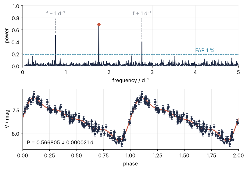
Top: Lomb-Scargle power against frequency, the peak at 1.76 per day above its one-day aliases and above the dashed 1 % false alarm line. Bottom: the light curve folded on the refined period with the four-harmonic model through it.

The period found is 0.5 s off the one put in, well inside its uncertainty of 1.8 s.

Pitfalls

A grid too coarse. The symptom is a period that is off by a lot, often onto an alias. The cause is a grid step wider than the peak, so the true peak falls between two grid points:

coarse = np.linspace(0.05, 5, 300)
print(f"step {coarse[1] - coarse[0]:.4f} 1/d, best period {1 / coarse[ls.power(coarse).argmax()]:.4f} d")

step 0.0166 1/d, best period 0.3617 d

A step of 0.0166 d⁻¹, twice the peak width, returns 0.3617 d, the alias at f + 1. Use samples_per_peak of 5 to 10, then refine around the peak as in Step 6.

Short nights make the alias win. The argument of Step 3 predicts that exposures bunched near midnight leave f and f ± 1 almost indistinguishable. Rerun the same seed with every exposure within half an hour of midnight, the same nights and the same noise:

rng_short = np.random.default_rng(144)
t_short = schedule(rng_short, half_night=0.5 / 24)
mag_short = rrlyrae_mag(t_short) + rng_short.normal(0, SIGMA, t_short.size)
p_short = LombScargle(t_short, mag_short, SIGMA).power(freq)
p_true = local_peak(p_short, 1 / P_TRUE)[1]
p_alias = max(local_peak(p_short, 1 / P_TRUE + s)[1] for s in (-1, 1))
print(f"alias / true peak: {p_alias / p_true:.3f} with ±0.5 h nights, "
      f"against {local_peak(power, f_best - 1)[1] / power.max():.3f} with ±4 h")

true_wins = 0
for seed in range(1, 21):                        # twenty other seasons, same short nights
    r = np.random.default_rng(seed)
    ts = schedule(r, half_night=0.5 / 24)
    p = LombScargle(ts, rrlyrae_mag(ts) + r.normal(0, SIGMA, ts.size), SIGMA).power(freq)
    true_wins += abs(freq[p.argmax()] - 1 / P_TRUE) < 0.02
print(f"the true peak wins in {true_wins} of 20 other seasons")

alias / true peak: 0.999 with ±0.5 h nights, against 0.740 with ±4 h
the true peak wins in 9 of 20 other seasons

The ratio climbs from 0.74 to 0.999. This season still picks the right peak, by a hair, and in twenty other seasons with short nights the true peak wins only nine times. Spread the exposures over the night, add a site at another longitude, and check the period against the physics: an RRab star at 1.31 d would be outside its class.

Reading the FAP as the probability that the period is right. The aliases are as significant as the peak:

for name, fc in [("f - 1", f_best - 1), ("f + 1", f_best + 1)]:
    p_peak = local_peak(power, fc)[1]
    print(f"{name}: power {p_peak:.2f}, FAP {ls.false_alarm_probability(p_peak, **limits):.0e}")

f - 1: power 0.51, FAP 2e-15
f + 1: power 0.40, FAP 2e-10

FAPs of 2 × 10⁻¹⁵ and 2 × 10⁻¹⁰ say that both are no accident of noise, and both are wrong. The FAP answers "is this noise", never "is this the period", and only for its own noise model: independent Gaussian errors with the relative sizes you passed, their overall scale fitted to the scatter.

Variations

A transiting planet. The dip in brightness is a box, which a sine fits badly; use astropy.timeseries.BoxLeastSquares with a grid of transit durations.
A circadian rhythm sampled at irregular hours. Times in hours, a search around 1/24 h⁻¹, and aliases set by the schedule, for example samples taken only during the working day.
A double-mode pulsator. Subtract the model at the first peak and run the periodogram on the residuals, a step called prewhitening, to find the second period.
Cycles in a sediment core. An age model turns depth into age, which gives uneven times, and the search runs in cycles per thousand years for the 41 kyr obliquity cycle.

Cheat sheet

ls = LombScargle(t, y, dy, nterms=1)                 # dy: uncertainties; nterms > 1 adds harmonics
freq, power = ls.autopower(minimum_frequency=fmin, maximum_frequency=fmax,
                           samples_per_peak=10)      # grid from the physics, step 1/(10 T)
power = ls.power(freq)                               # on a grid of your own, e.g. a fine one
fap = ls.false_alarm_probability(power.max(), minimum_frequency=fmin, maximum_frequency=fmax)
level = ls.false_alarm_level(0.01, minimum_frequency=fmin, maximum_frequency=fmax)
window = LombScargle(t, np.ones_like(t), fit_mean=False, center_data=False).power(freq)  # ones survive
phase = (t * f) % 1                                  # fold; compare folds on f and f ± 1
y_model = ls.model(t_fit, f)                         # the fitted curve at any times