Malmquist bias: why the stars in a catalog are brighter than their type

The question

A catalog lists every star brighter than apparent magnitude 12, and 23,125 of its stars belong to one type. Star clusters at known distances say that the type has a mean absolute magnitude of +1.00 with a Gaussian scatter of 0.5 mag. Give each catalog star its true distance and the average absolute magnitude comes out +0.66, a third of a magnitude brighter than the type. That shift is the Malmquist bias of a magnitude-limited, or flux-limited, catalog, and it appears although every star was measured perfectly.

Astronomers measure brightness backwards and logarithmically. The apparent magnitude \(m\) measures the flux that arrives: smaller is brighter, and 5 mag is a factor of 100 in flux. The absolute magnitude \(M\) is the apparent magnitude a star would have at 10 pc, so it measures the star's luminosity and does not depend on where the star is. The two are linked by the distance modulus, \(m - M = 5\log_{10}(d / 10\,\mathrm{pc})\). How the stars of a type are spread over \(M\), the number per unit \(M\), is the luminosity function \(\varphi(M)\); here it is a Gaussian with mean \(M_0\) and width \(\sigma\), and it has nothing to do with a spectrum.

The catalog is simulated, because only a simulation knows every star's true \(M\). One million stars fill a sphere of radius 6 kpc around the observer uniformly. The share of them within radius \(r\) is then \((r/R)^3\), so radii \(r = R\,u^{1/3}\) with \(u\) uniform on \([0, 1)\) place them correctly (inverse transform sampling). Each star draws its \(M\) from the Gaussian and gets its \(m\) from the distance modulus, and it enters the catalog if \(m < 12\). There is no dust and no measurement error.

Show code

Copy

import numpy as np
import matplotlib.pyplot as plt

plt.rcParams.update({
    "figure.figsize": (7, 3.6), "figure.dpi": 110,
    "axes.spines.top": False, "axes.spines.right": False,
    "axes.grid": True, "grid.alpha": 0.25,
    "font.size": 11, "lines.linewidth": 1.8,
})
INK, ACCENT, SECOND, MUTED = "#1f2a44", "#c8553d", "#2a7f9e", "#8a8f98"

M0, SIGMA = 1.0, 0.5             # the type: mean absolute magnitude and scatter / mag
M_LIM = 12.0                     # the catalog's limit in apparent magnitude
R_PC, N = 6000.0, 1_000_000      # radius of the population / pc, number of stars

# The draw order is fixed: radii first, then magnitudes. Every number in the text depends on it.
rng = np.random.default_rng(42)
d = R_PC * rng.random(N) ** (1 / 3)          # pc, uniform in the volume of the sphere
M = rng.normal(M0, SIGMA, N)
m = M + 5 * np.log10(d / 10)
seen = m < M_LIM

print(f"population: {N:,} stars    catalog (m < {M_LIM:.0f}): {seen.sum():,} stars, "
      f"{seen.mean():.1%} of the population")
print(f"catalog: mean M = {M[seen].mean():+.3f} mag, standard deviation {M[seen].std():.3f} mag")

bins = np.arange(-1.0, 3.01, 0.1)
fig, ax = plt.subplots()
ax.hist(M[seen], bins, density=True, color=ACCENT, alpha=0.35, lw=0)
ax.hist(M[seen], bins, density=True, histtype="step", color=ACCENT, lw=1.2)
ax.axvline(M0, color=MUTED, lw=1.2, ls="--")
ax.axvline(M[seen].mean(), color=ACCENT, lw=1.2)
ax.text(M0 + 0.04, 0.9, f"type, M₀ = {M0:+.2f}", color=MUTED, va="center")
ax.text(M[seen].mean() - 0.04, 0.9, f"catalog, {M[seen].mean():+.2f}", color=ACCENT, ha="right",
        va="center")
ax.annotate("brighter", (-0.9, 0.55), xytext=(-0.3, 0.55), va="center", color=MUTED,
            arrowprops=dict(arrowstyle="->", color=MUTED, lw=1))
ax.set(xlabel="absolute magnitude M / mag", ylabel="density / 1/mag", xlim=(-1, 3), ylim=(0, 0.97))
plt.show()

population: 1,000,000 stars    catalog (m < 12): 23,125 stars, 2.3% of the population
catalog: mean M = +0.659 mag, standard deviation 0.498 mag

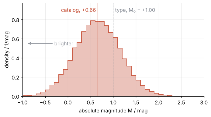
The histogram is a Gaussian of the right width, 0.50 mag, holding 2.3 % of the million stars, and it sits 0.34 mag to the bright side of the type's mean, the dashed line.

Where does the shift come from, when every star drew its \(M\) from the same Gaussian? And a star of known type is a standard candle: its distance follows from its \(m\) and the type's mean. How wrong is that distance for a catalog star?

The idea: bright stars are seen in a bigger volume

A star of absolute magnitude \(M\) stays brighter than the limit out to the distance where its apparent magnitude reaches 12, \(d_{\max}(M) = 10\,\mathrm{pc}\cdot 10^{0.2(12 - M)}\). Brighter stars are visible farther away, and the volume in which they are visible grows with the cube of that distance. A catalog is not a sample of the stars. It is a sample of the volumes in which they can be seen.

def d_max(M_abs, m_lim=M_LIM):
    """Distance / pc out to which a star of absolute magnitude M_abs is brighter than m_lim."""
    return 10 * 10 ** (0.2 * (m_lim - M_abs))

for dM in [0.0, -0.5, -1.0]:
    print(f"M = {M0 + dM:+.2f}:  d_max = {d_max(M0 + dM) / 1000:.2f} kpc,  "
          f"volume {(d_max(M0 + dM) / d_max(M0)) ** 3:.2f} times that of the type's mean")

M = +1.00:  d_max = 1.58 kpc,  volume 1.00 times that of the type's mean
M = +0.50:  d_max = 2.00 kpc,  volume 2.00 times that of the type's mean
M = +0.00:  d_max = 2.51 kpc,  volume 3.98 times that of the type's mean

A star at the type's mean is caught out to 1.58 kpc. One 0.5 mag brighter is caught out to 2.00 kpc, in twice the volume, and one a full magnitude brighter in 3.98 times the volume. Plot absolute magnitude against distance for 20,000 of the million and the cut appears as a diagonal line. The magnitude axis runs downward, bright at the top, as astronomers draw it.

Show code

Copy

sample = slice(0, 20_000)        # the first 20,000 stars are already a random sample
fig, ax = plt.subplots(figsize=(7, 3.8))
ax.plot(d[sample][~seen[sample]], M[sample][~seen[sample]], "o", ms=1.5, color=INK, alpha=0.3, mew=0)
ax.plot(d[sample][seen[sample]], M[sample][seen[sample]], "o", ms=2, color=ACCENT, mew=0)
d_line = np.geomspace(130, R_PC, 200)
ax.plot(d_line, M_LIM - 5 * np.log10(d_line / 10), color=SECOND, lw=1.6)
ax.text(2.4e3, -0.85, f"m = {M_LIM:.0f}", color=SECOND, ha="right")
ax.set(xscale="log", xlim=(130, R_PC), ylim=(3.2, -1.2),          # the nearest star of the sample is at 142 pc
       xlabel="distance / pc", ylabel="absolute magnitude M / mag")
ax.set_xticks([200, 500, 1000, 2000, 5000], ["200", "500", "1,000", "2,000", "5,000"])
ax.set_xticks([], minor=True)
plt.show()

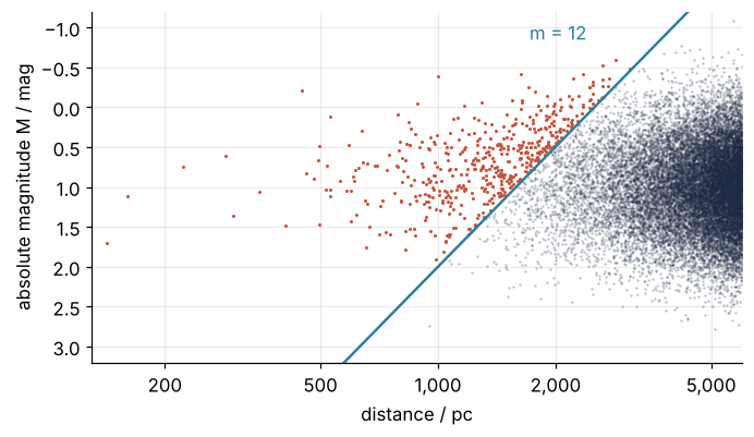
Near the Sun every star is above the line and in the catalog, whatever its \(M\). Beyond 2 kpc only the bright tail is left, and that is where most of the population lives, because the outer shells of a sphere hold most of its volume.

The number of catalog stars at a given \(M\) is the number in the population at that \(M\) times the volume in which they are seen. The volume factor is \(d_{\max}^3 \propto 10^{-0.6M}\), three times the 0.2 of the distance. Multiply the Gaussian luminosity function by it and the product is the distribution the catalog sees. Here it is for three widths of the Gaussian:

Show code

Copy

M_grid = np.linspace(-4, 4, 4001)
fig, axes = plt.subplots(3, 1, figsize=(7, 6.3), sharex=True)
for ax, s in zip(axes, [0.25, 0.5, 1.0]):
    phi = np.exp(-0.5 * ((M_grid - M0) / s) ** 2)
    volume = 10 ** (-0.6 * M_grid)
    product = phi * volume
    shift = np.sum(M_grid * product) / np.sum(product) - M0
    ax.plot(M_grid, phi, color=INK, label="population")
    ax.plot(M_grid, volume / volume[np.searchsorted(M_grid, M0)] * 0.5, color=SECOND, lw=1.1,
            label="volume factor")
    ax.fill_between(M_grid, product / product.max(), color=ACCENT, alpha=0.35, lw=0, label="catalog")
    ax.text(0.99, 0.9, f"σ = {s:.2f} mag\nshift {shift:+.2f} mag".replace("-", "−"), transform=ax.transAxes,
            ha="right", va="top")
    ax.set(ylim=(0, 1.15), ylabel="relative")
axes[0].legend(frameon=False, loc="upper left")
axes[-1].set(xlabel="absolute magnitude M / mag", xlim=(-3, 4))
plt.show()

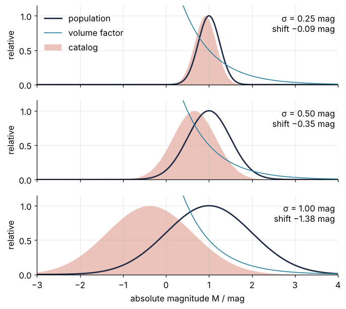
The product is again a Gaussian of the same width, slid to the bright side, not skewed. Its shift is −0.09 mag for \(\sigma\) = 0.25 mag, −0.35 mag for 0.5, and −1.38 mag for 1.0: four times larger for every doubling of the scatter, so the shift grows as \(\sigma^2\). A type with a scatter of a full magnitude is off by more than its own scatter.

A fainter limit does not remove the bias, until the survey runs out of stars

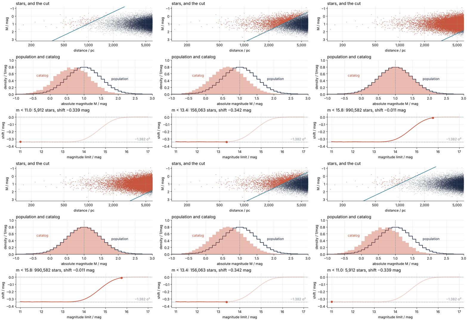
A deeper survey looks as if it should help, since it catches more of the faint stars. In a population without an edge it does not: moving the limit from 12 to 13 multiplies every \(d_{\max}\) by the same factor 1.58, and the ratios between the volumes of bright and faint stars stay as they were. The simulated population does have an edge, at 6 kpc, and sweeping the limit shows what that does.

for lim in range(11, 18):
    cut = m < lim
    print(f"m < {lim}:  {cut.sum():>9,} stars   shift {M[cut].mean() - M0:+.3f} mag")

m < 11:      5,912 stars   shift -0.339 mag
m < 12:     23,125 stars   shift -0.341 mag
m < 13:     92,849 stars   shift -0.343 mag
m < 14:    356,922 stars   shift -0.308 mag
m < 15:    854,405 stars   shift -0.108 mag
m < 16:    997,371 stars   shift -0.003 mag
m < 17:    999,998 stars   shift +0.001 mag

From \(m < 11\) to \(m < 13\) the catalog grows sixteenfold, from 5,912 to 92,849 stars, and the shift stays at −0.34 mag. It falls once the bright stars reach the edge of the sphere and a deeper limit has no more volume to give them. At \(m < 14\) every star brighter than \(M = +0.11\) is already visible out to 6 kpc, and the shift is −0.308 mag; it is −0.108 at 15, and −0.003 at 16, where the catalog holds 997,371 of the million stars.

"""Limit sweep: the Malmquist shift of a magnitude-limited catalog as the limit gets fainter.

Renders ../../assets/limit-sweep.gif from the population of the tutorial (same constants,
same seed). Run it from any directory:

    python scene.py
"""
from pathlib import Path

import numpy as np
import matplotlib.pyplot as plt
from matplotlib.animation import FuncAnimation, PillowWriter
from PIL import Image

OUT = Path(__file__).resolve().parents[2] / "assets" / "limit-sweep.gif"
INK, ACCENT, SECOND, MUTED = "#1f2a44", "#c8553d", "#2a7f9e", "#8a8f98"
plt.rcParams.update({"axes.spines.top": False, "axes.spines.right": False,
                     "axes.grid": True, "grid.alpha": 0.25, "font.size": 11})

# ---- data: the population of the tutorial, and the shift for every limit
M0, SIGMA, R_PC, N = 1.0, 0.5, 6000.0, 1_000_000
rng = np.random.default_rng(42)
d = R_PC * rng.random(N) ** (1 / 3)                                  # pc, uniform in the sphere
M = rng.normal(M0, SIGMA, N)
m = M + 5 * np.log10(d / 10)

# The limit runs from 11 to 17 and back, with a short hold at each end, so the loop has no seam.
sweep = np.linspace(11, 17, 54)
frames = np.concatenate([sweep, [17] * 4, sweep[-2:0:-1], [11] * 4])   # 114 frames
shift_sweep = np.array([M[m < lim].mean() - M0 for lim in sweep])     # the shift along the sweep
bins = np.arange(-1.0, 3.01, 0.1)
pop_hist, _ = np.histogram(M, bins, density=True)
shown = slice(0, 20_000)                                             # stars drawn, as in the notebook

# ---- figure, drawn once
fig, (ax1, ax2, ax3) = plt.subplots(3, 1, figsize=(7, 7.2), dpi=80, layout="constrained")
ax1.scatter(d[shown], M[shown], s=2, color=INK, alpha=0.3, lw=0)
seen_dots = ax1.scatter([], [], s=2, color=ACCENT, lw=0)
d_line = np.geomspace(130, R_PC, 200)
(cut_line,) = ax1.plot([], [], color=SECOND, lw=1.6)
ax1.set(xscale="log", xlim=(130, R_PC), ylim=(3.2, -1.2),          # the nearest shown star is at 142 pc
        xlabel="distance / pc", ylabel="M / mag")
ax1.set_xticks([200, 500, 1000, 2000, 5000], ["200", "500", "1,000", "2,000", "5,000"])
ax1.set_xticks([], minor=True)
ax2.stairs(pop_hist, bins, color=INK, lw=1.6)
cat_steps = ax2.stairs(pop_hist, bins, fill=True, color=ACCENT, alpha=0.4, lw=0)
ax2.axvline(M0, color=MUTED, lw=1, ls="--")
ax2.set(xlim=(bins[0], bins[-1]), ylim=(0, 1.0), xlabel="absolute magnitude M / mag",
        ylabel="density / 1/mag")
ax2.text(-0.05, 0.55, "catalog", color=ACCENT, ha="right", va="center")
ax2.text(1.8, 0.45, "population", color=INK, va="center")
ax3.axhline(-0.6 * np.log(10) * SIGMA**2, color=MUTED, lw=1, ls="--")
ax3.axhline(0, color=MUTED, lw=1, ls="--")
ax3.text(17.1, -0.6 * np.log(10) * SIGMA**2 + 0.012, "−1.382 σ²", color=MUTED, ha="right", va="bottom")
ax3.plot(sweep, shift_sweep, color=ACCENT, lw=1.8, alpha=0.3)        # the whole curve, faint
(trace,) = ax3.plot([], [], color=ACCENT, lw=1.8)                    # solid up to the current limit
(dot,) = ax3.plot([], [], "o", color=ACCENT, ms=6)
ax3.set(xlim=(10.8, 17.2), ylim=(-0.42, 0.05), xlabel="magnitude limit / mag",
        ylabel="shift / mag")
ax1.set_title("stars, and the cut", loc="left")
ax2.set_title("population and catalog", loc="left")
title3 = ax3.set_title("", loc="left")

# ---- one frame: a function of the limit alone
def update(i):
    lim = frames[i]
    seen = m < lim
    shift = M[seen].mean() - M0
    keep = seen[shown]
    seen_dots.set_offsets(np.column_stack([d[shown][keep], M[shown][keep]]))
    cut_line.set_data(d_line, lim - 5 * np.log10(d_line / 10))     # where m equals the limit
    cat_hist, _ = np.histogram(M[seen], bins, density=True)
    cat_steps.set_data(cat_hist)
    upto = sweep <= lim + 1e-9
    trace.set_data(sweep[upto], shift_sweep[upto])
    dot.set_data([lim], [shift])
    title3.set_text(f"m < {lim:.1f}: {seen.sum():,} stars, shift {shift:+.3f} mag".replace("-", "−"))

# ---- render, and read back what was written
OUT.parent.mkdir(exist_ok=True)
FuncAnimation(fig, update, frames=len(frames)).save(OUT, writer=PillowWriter(fps=12))
plt.close(fig)
with Image.open(OUT) as im:
    seconds = len(frames) / 12                                       # Pillow merges repeated frames
    print(f"{OUT.name}: {im.width} x {im.height} px, {len(frames)} frames at 12 fps, "
          f"{seconds:.1f} s, {OUT.stat().st_size / 1024:,.0f} kB")

The return to zero is not a reward for depth. Once the bright stars sit at the edge, each deeper limit adds only fainter ones, and they catch up. What sets the bias is the cut together with how the stars fill space, and the survey's depth matters only through that.

Formalization

The figures all computed the same quantity. The number of catalog stars per unit \(M\) is the luminosity function times the density of stars times the volume in which a star of that \(M\) passes the cut:

with \(\rho\) the number of stars per unit volume, constant here. Write the volume factor as an exponential, \(10^{-0.6M} = e^{-aM}\) with \(a = 0.6\ln 10\), and add it to the exponent of the Gaussian. Completing the square gives

a Gaussian of the same width \(\sigma\), centered at \(M_0 - a\sigma^2\). That is the result Malmquist published in 1922:

where \(\langle M \rangle_{\text{cat}}\) is the mean absolute magnitude of the whole catalog. Three consequences follow.

The size. For \(\sigma\) = 0.5 mag the bias is \(1.382 \times 0.25 = 0.345\) mag; for 0.25 mag it is 0.086, for 1 mag it is 1.38. Neither the limit nor \(\rho\) appears in the formula, which is the plateau of the sweep: as long as the population has no edge within reach, a catalog of 6,000 stars and one of 90,000 carry the same bias.

Distances come out short, and for galaxies the Hubble constant too large. The distance computed from the type's mean is \(d = 10\,\mathrm{pc}\cdot 10^{0.2(m - M_0)}\), and against the true distance it is off by the factor \(10^{0.2(M - M_0)}\). For the median catalog star, whose \(M\) is the catalog's mean, that is \(10^{-0.2 \times 0.345} = 0.853\): 15 % short. The stars of this catalog lie within 6 kpc and take no part in the expansion of the universe, but galaxies do, and they are used the same way. The Tully-Fisher relation gives a spiral galaxy's luminosity from its rotation speed, which makes it a star of known type at tens of Mpc. In a magnitude-limited sample of such galaxies the distances are short by the same factor, and the Hubble constant from Hubble's law \(v = H_0 d\), the recession velocity proportional to distance, comes out \(1/0.853 = 1.17\) times too large, by 17 %.

How the stars fill space decides. A constant \(\rho\) cancels, but the way the stars spread through space does not: the derivation used one fact about it, that the volume within \(d\) grows as \(d^3\). Put the stars in a thin flat sheet instead, with the observer at its center and in its plane, and the stars of magnitude \(M\) that pass the cut fill a disk of area \(\pi d_{\max}^2 \propto 10^{-0.4M}\). The same square gives \(0.4\ln 10\,\sigma^2 = 0.921\,\sigma^2\), which is 0.230 mag for \(\sigma\) = 0.5 mag: each dimension the stars spread in adds \(0.2\ln 10\,\sigma^2 = 0.46\,\sigma^2\). The simulation in the sheet places radii at \(r = R\sqrt{u}\), the area version of the cube root above:

# Stars uniform in a flat disk of radius R, the observer at its center and in its plane.
r_sheet = R_PC * np.sqrt(rng.random(N))
M_sheet = rng.normal(M0, SIGMA, N)
seen_sheet = M_sheet + 5 * np.log10(r_sheet / 10) < M_LIM
n_sheet = seen_sheet.sum()
print(f"sheet: {n_sheet:,} stars in the catalog, shift "
      f"{M_sheet[seen_sheet].mean() - M0:+.3f} ± {SIGMA / np.sqrt(n_sheet):.3f} mag, "
      f"theory {-0.4 * np.log(10) * SIGMA**2:+.3f} mag")

sheet: 77,635 stars in the catalog, shift -0.231 ± 0.002 mag, theory -0.230 mag

The simulated sheet gives −0.231 ± 0.002 mag against −0.230 predicted. At the other extreme sits a cluster, every member at one distance: \(V(M)\) is the same for every \(M\), and when the whole cluster is brighter than the limit the shift is zero. That is why clusters calibrate \(M_0\) in the first place; a limit that cuts into the cluster's Gaussian truncates it instead, which is a different bias. Correcting a real catalog therefore needs a model of how its stars fill space, and that model is where the arguments are.

See it in code

The measurement on the catalog of the first cell, with the standard error \(\sigma/\sqrt{n}\) as the error bar (The standard error of the mean) and twenty more seeded generators (Random numbers with numpy.random) to see how much the shift scatters between catalogs:

Show code

Copy

n = seen.sum()
shift = M[seen].mean() - M0
predicted = -0.6 * np.log(10) * SIGMA**2
d_from_M0 = 10 * 10 ** (0.2 * (m - M0))
ratio = d_from_M0[seen] / d[seen]


def catalog_shift(seed):
    g = np.random.default_rng(seed)
    dd = R_PC * g.random(N) ** (1 / 3)
    MM = g.normal(M0, SIGMA, N)
    return MM[MM + 5 * np.log10(dd / 10) < M_LIM].mean() - M0


others = np.array([catalog_shift(seed) for seed in range(20)])
print(f"catalog:            {n:,} stars, mean M = {M[seen].mean():+.3f} mag")
print(f"shift:              {shift:+.3f} ± {SIGMA / np.sqrt(n):.3f} mag   (-1.382 σ² = {predicted:+.3f})")
print(f"twenty other seeds: mean {others.mean():+.3f} mag, scatter {others.std(ddof=1):.4f} mag")
print(f"brightest star:     M = {M.min():+.2f} mag, visible to {d_max(M.min()) / 1000:.1f} kpc "
      f"< R = {R_PC / 1000:.0f} kpc")
spread = 0.2 * np.log(10) * SIGMA            # standard deviation of ln(ratio)
print(f"distance from M0:   median {np.median(ratio):.3f} of the true one (theory {10 ** (0.2 * predicted):.3f}), "
      f"mean {ratio.mean():.3f} (theory {10 ** (0.2 * predicted) * np.exp(spread**2 / 2):.3f})")
print(f"H0 too large by:    {1 / 10 ** (0.2 * predicted):.2f} from distance moduli, "
      f"{np.mean(1 / ratio):.2f} averaging v/d galaxy by galaxy")

fig, (ax1, ax2) = plt.subplots(2, 1, figsize=(7, 4.4), layout="constrained")
ax1.hist(M[seen], bins, density=True, color=ACCENT, alpha=0.35, lw=0)
ax1.stairs(np.histogram(M, bins, density=True)[0], bins, color=INK, lw=1.6)
ax1.text(0.99, 0.95, f"measured {shift:+.3f} ± {SIGMA / np.sqrt(n):.3f} mag\n"
         f"1.382 σ² predicts {predicted:+.3f} mag".replace("-", "−"), transform=ax1.transAxes,
         ha="right", va="top")
ax1.text(-0.05, 0.55, "catalog", color=ACCENT, ha="right", va="center")
ax1.text(1.8, 0.45, "population", color=INK, va="center")
ax1.set(xlabel="absolute magnitude M / mag", ylabel="density / 1/mag", xlim=(-1, 3), ylim=(0, 1.0))
counts, _, _ = ax2.hist(ratio, np.linspace(0.5, 1.5, 61), color=ACCENT, alpha=0.35, lw=0)
ax2.axvline(1, color=MUTED, lw=1, ls="--")
ax2.axvline(np.median(ratio), color=ACCENT, lw=1.2)
ax2.text(np.median(ratio) - 0.01, 0.97, f"median {np.median(ratio):.3f}", color=ACCENT, ha="right",
         va="top", transform=ax2.get_xaxis_transform())
ax2.set(xlabel="distance from M₀ / true distance", ylabel="stars", xlim=(0.5, 1.5),
        ylim=(0, 1.2 * counts.max()))
plt.show()

catalog:            23,125 stars, mean M = +0.659 mag
shift:              -0.341 ± 0.003 mag   (-1.382 σ² = -0.345)
twenty other seeds: mean -0.346 mag, scatter 0.0032 mag
brightest star:     M = -1.54 mag, visible to 5.1 kpc < R = 6 kpc
distance from M0:   median 0.854 of the true one (theory 0.853), mean 0.877 (theory 0.876)
H0 too large by:    1.17 from distance moduli, 1.20 averaging v/d galaxy by galaxy

The measured shift, −0.341 ± 0.003 mag, lies about one standard error from Malmquist's −0.345, and twenty other seeds scatter by 0.0032 mag around a mean of −0.346, as large as the error bar says. The brightest of the million stars is visible to 5.1 kpc, inside the 6 kpc edge, so the edge did not touch the catalog at \(m < 12\). The median distance ratio, 0.854, agrees with \(10^{-0.2 \times 0.345} = 0.853\) to the third digit.

The mean ratio, 0.877, is larger, and it should be. The ratio is \(10^{0.2(M - M_0)}\), 10 raised to a Gaussian variable, which makes it lognormal, and its histogram has a longer tail to the right of the median than to the left. The tail pulls the mean up by the factor \(e^{s^2/2}\), with \(s = 0.2\ln 10\,\sigma\) the width of the ratio's logarithm, which turns 0.853 into the 0.876 printed. Malmquist's bias is a shift in magnitudes, and it converts to the median ratio, not the mean. Average in magnitudes, as astronomers do when they fit a Hubble diagram, and the 1.17 on \(H_0\) is the answer; average \(v/d\) galaxy by galaxy and you get 1.20, the bias plus the spread.

Where it shows up

• Extragalactic astronomy. Tully-Fisher distances to galaxies in a magnitude-limited sample come out short, and the Hubble constant too large, as in the second consequence. That factor comes from the shift of the whole sample: at a fixed distance the bias is zero close in, where every galaxy passes the limit, and grows outward, where only the luminous ones do, so the distant galaxies inflate \(H_0\) most. Teerikorpi's 1997 review traces how this bias ran through the debate over the extragalactic distance scale from the 1970s to the 1990s.
• Astrometry. Parallaxes carry measurement errors, and there are more stars at small true parallax than at large, so a sample selected by measured parallax holds more stars scattered up from smaller parallaxes than down from larger ones. Those stars are on average farther than their measured parallax says and their luminosities come out too faint: the Lutz-Kelker bias, described by Lutz and Kelker in 1973.
• Planetary science. A transit survey such as Kepler finds a planet when the dip in the star's light beats the noise, and a large planet beats the noise around fainter, noisier stars than a small one can. Large planets are therefore found among more stars and are over-represented in the raw counts, until the survey's completeness is measured by injecting artificial transits into the data.
• Seismology. A network detects a small earthquake only near a station and a large one across a continent, so the area in which an event is caught grows with its magnitude, and the poorly covered parts of a regional catalog are full of large events. Seismologists cut a catalog at its magnitude of completeness, \(M_c\), above which every event is recorded, for exactly this reason.
• Particle physics. A trigger keeps an event when its measured energy passes a threshold, so near the threshold it keeps the events whose energy fluctuated up and loses those that fluctuated down. The measured spectrum near threshold is biased high, the effect known as Eddington bias after his 1913 paper, with measurement noise in place of intrinsic scatter.
• Medicine. A hospital study sees only the patients ill enough to be admitted, and a patient with two conditions is more likely to be admitted than one with either alone. Two diseases unrelated in the population then look associated among the inpatients, which is Berkson's bias of 1946.

None of these goes away in a larger sample, and every repair, whether a weight, a prior, an unfolding, or a stricter cut, starts from a model of which objects could have passed the cut.

Further reading

• numpy.random.Generator for the seeded generator and its distributions.
• K. G. Malmquist (1922), Lund Meddelanden, Ser. I, No. 100, for the original result; P. Teerikorpi (1997), "Observational selection bias affecting the determination of the extragalactic distance scale", Annual Review of Astronomy and Astrophysics 35, 101, for its history in cosmology.
• J. Binney and M. Merrifield, Galactic Astronomy (Princeton, 1998), for the bias in star counts and its corrections.
• Related tutorials on this site: The standard error of the mean, Inverse transform sampling, Random numbers with numpy.random, and Multiple testing, another way a fair-looking sample misleads.
• Download the notebook. It was executed with the library versions in the header.