Multiple testing: why ten thousand t-tests find hundreds of false discoveries

The question

An expression screen measures 10,000 genes in treated and control cells, three replicates per group, and runs one t-test per gene. Here is the result as biologists draw it, a volcano plot with one dot per gene:

Show code

Copy

import numpy as np
import matplotlib.pyplot as plt
from scipy import stats

plt.rcParams.update({
    "figure.figsize": (7, 3.6), "figure.dpi": 110,
    "axes.spines.top": False, "axes.spines.right": False,
    "axes.grid": True, "grid.alpha": 0.25,
    "font.size": 11, "lines.linewidth": 1.8,
})
INK, ACCENT, SECOND, MUTED = "#1f2a44", "#c8553d", "#2a7f9e", "#8a8f98"

# The screen is simulated from a known truth, so that every answer can be checked.
M, M1, N, SD, LFC = 10_000, 500, 3, 0.3, 2.0     # genes, responders, replicates, noise and shift in log2 units

def simulate_screen(rng):
    """Log2 expression of M genes, N replicates per group; the first M1 genes respond."""
    baseline = rng.normal(8, 1.5, (M, 1))
    control = baseline + rng.normal(0, SD, (M, N))
    treated = baseline + rng.normal(0, SD, (M, N))
    sign = rng.choice([-1, 1], M1)                # fourfold up or fourfold down
    treated[:M1] += (sign * LFC)[:, None]
    return control, treated

control, treated = simulate_screen(np.random.default_rng(2026))
responder = np.arange(M) < M1
p = stats.ttest_ind(treated, control, axis=1).pvalue      # axis=1: one test per row, that is per gene
fold = treated.mean(axis=1) - control.mean(axis=1)

fig, ax = plt.subplots()
ax.plot(fold, -np.log10(p), "o", color=INK, ms=2, alpha=0.4, mew=0)
ax.axhline(-np.log10(0.05), color=MUTED, lw=1, ls="--")
ax.text(3.4, -np.log10(0.05) + 0.15, "p = 0.05", color=MUTED, ha="right", va="bottom")
ax.text(0, 6.6, f"{(p < 0.05).sum():,} genes above the line", color=INK, ha="center", va="top")
ax.set(xlabel="fold change, log2 (1 = twice as much)", ylabel="−log10 p (higher = smaller p)",
       xlim=(-3.5, 3.5))
plt.show()
print(f"genes with p < 0.05: {(p < 0.05).sum():,} of {M:,}")

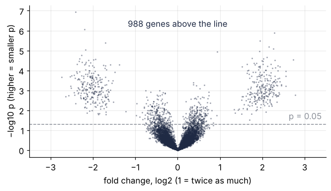
genes with p < 0.05: 988 of 10,000

Expression is on a log2 scale, so a fold change of 1 means the gene doubled and ±2 means fourfold up or down. The height is −log10 p, so a smaller p sits higher: p = 0.05 is at 1.3 and p = 10⁻⁶ at 6. Significant is up, a large change is out to either side, and the interesting genes sit in the two upper corners. The dashed line marks p = 0.05, and every dot above it passes the test that a single experiment with one gene would be judged by.

Two things are obvious. There are two arms of strong hits near ±2, and there is a dense cloud of small changes around zero whose top reaches above the dashed line. Together, 988 genes have p < 0.05.

Less obvious: how many of the 988 are real? The data are simulated with a known truth, 500 genes that respond and 9,500 that do not, so every answer here can be checked against it. Each of the 10,000 p-values is computed correctly. The trouble is what a p-value promises for one test and does not promise for ten thousand, and the question of this tutorial is how to build a hit list whose share of false hits you control.

The idea: p-values of null genes are uniform

Take one gene that does not respond. Its treated and control values are the same baseline plus noise, and the t-test asks how surprising the observed difference would be if that were so. The p-value is built so that a difference exceeded by 5 % of such null experiments gets p = 0.05, one exceeded by 1 % gets p = 0.01, and so on all the way down. So among many null genes, 5 % have p below 0.05, 1 % below 0.01, and a share x below any x between 0 and 1. That is what "uniform on [0, 1]" means, and it is all that "p < 0.05 happens 5 % of the time when nothing is there" says.

A threshold of 0.05 therefore keeps 5 % of the 9,500 null genes, about 475, whichever they are. Check it on the screen:

p_null, p_real = p[~responder], p[responder]
for alpha in [0.05, 0.01]:
    print(f"share of null genes below {alpha:.2f}: {np.mean(p_null < alpha):.4f}   "
          f"({np.sum(p_null < alpha)} of {p_null.size:,})")

# the prerequisite's default, Welch's test, on the same genes
p_welch = stats.ttest_ind(treated, control, axis=1, equal_var=False).pvalue
print(f"Welch's test, share below 0.05:    {np.mean(p_welch[~responder] < 0.05):.4f}")

share of null genes below 0.05: 0.0514   (488 of 9,500)
share of null genes below 0.01: 0.0115   (109 of 9,500)
Welch's test, share below 0.05:    0.0373

Of the 9,500 null genes, 5.1 % fall below 0.05 and 1.1 % below 0.01, as promised. That holds for Student's test, which this screen uses because its noise is equal in both groups by construction. Welch's test, the prerequisite's default, puts only 3.7 % below 0.05. With equal group sizes its t is the same number as Student's, judged with fewer degrees of freedom, so no p-value comes out smaller. At three replicates the difference is large.

On a real screen, where nobody guarantees equal noise, keep Welch. With unequal noise and three replicates Welch's null p-values are not exactly uniform either, so the false share promised in the next section becomes a target, not a guarantee.

Split all the p-values by the truth and draw a histogram of each, with bins of width 0.05:

Show code

Copy

bins = np.linspace(0, 1, 21)
fig, (ax1, ax2) = plt.subplots(2, 1, figsize=(7, 4.4), sharex=True)
ax1.hist(p_null, bins=bins, color=ACCENT, alpha=0.85, lw=0)
ax1.axhline(p_null.size / 20, color=MUTED, lw=1, ls="--")
ax1.text(0.005, 535, f"{p_null.size // 20} per bin", color=MUTED, va="bottom")
ax1.text(0.99, 0.95, "9,500 null genes", transform=ax1.transAxes, ha="right", va="top", color=ACCENT)
ax1.set(ylabel="genes per bin", ylim=(0, 650))
ax2.hist(p_real, bins=bins, color=INK, alpha=0.85, lw=0)
for ax in (ax1, ax2):
    ax.set_axisbelow(True)                         # grid behind the bars
ax2.text(0.99, 0.95, "500 responders", transform=ax2.transAxes, ha="right", va="top", color=INK)
ax2.set(xlabel="p-value", ylabel="genes per bin", xlim=(0, 1), ylim=(0, 560))
plt.show()

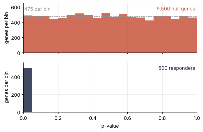
The null genes form a flat floor at about 475 per bin, the dashed line. The responders all sit in the first bin. A hit list at p < 0.05 is that first bin of both panels added together, 500 real genes and 488 null ones, and nothing in the list tells them apart.

The responders crowd into the first bin because their shift of 2 log2 units is 6.7 times the replicate noise of 0.3. That is a clean cell-line screen with strong responders, not a typical one: in scipy.stats from the ground up, only 45 % of the runs found a real difference at twelve batches. Weaker responders spread over the first several bins and mix with the floor.

Sorting the p-values: the Benjamini-Hochberg line

A fixed threshold ignores how many tests there are. It keeps 5 % of the null genes whether there are 20 of them or 9,500. The way out starts with sorting: put the 10,000 p-values in increasing order and plot the k-th smallest against its rank k.

If m p-values are spread evenly between 0 and 1, about k of them lie below k/m, so the k-th smallest sits near k/m. Against rank, that is a straight line of slope 1/m. Real effects have p-values far smaller than their rank predicts, and they pull the start of the curve down toward zero.

The rule of Benjamini and Hochberg draws a second line from the origin, k·q/m, with q times that slope. The largest rank at which the sorted p-values still lie below this line sets the cutoff, and every gene to its left is a discovery.

The number q is the share of false hits you accept in the list you will follow up: at q = 0.05, on average at most one hit in twenty is noise. A q of 0.05 or 0.1 is usual when every hit gets checked by a second experiment, and smaller when each follow-up costs a month of work. Choose it before you look at the list, not after. Here are the first 800 ranks with the line at a strict, a usual, and a generous q:

Show code

Copy

order = np.argsort(p)
p_sorted, true_sorted = p[order], responder[order]
rank = np.arange(1, M + 1)

def bh_count(q):
    """Largest rank whose sorted p-value lies on or below the line rank * q / M."""
    under = np.nonzero(p_sorted <= rank * q / M)[0]
    return under[-1] + 1 if under.size else 0

show = rank <= 800
fig, ax = plt.subplots()
ax.plot(rank[show], p_sorted[show], "o", color=MUTED, ms=2.5, mew=0)
for q, alpha in [(0.01, 0.4), (0.05, 0.7), (0.2, 1.0)]:
    k = bh_count(q)
    ax.plot([0, 800], [0, 800 * q / M], color=SECOND, lw=1.2, alpha=alpha)
    ax.plot(k, k * q / M, "o", ms=6, mfc="none", mec=SECOND, mew=1.2, zorder=4)   # the cutoff
    ax.text(810, 800 * q / M, f"q = {q}: {k} genes", color=SECOND, va="center")
k = bh_count(0.2)                                  # color the q = 0.2 list by the truth
found = rank <= k
ax.plot(rank[found & true_sorted], p_sorted[found & true_sorted], "o", color=INK, ms=2.5, mew=0)
ax.plot(rank[found & ~true_sorted], p_sorted[found & ~true_sorted], "o", color=ACCENT, ms=2.5, mew=0)
for y, label, color in [(0.019, "in the q = 0.2 list, true", INK), (0.0168, "in the q = 0.2 list, false", ACCENT),
                        (0.0146, "not in the list", MUTED)]:
    ax.text(15, y, label, color=color, va="top")
ax.set(xlabel="rank k", ylabel="k-th smallest p", xlim=(0, 800), ylim=(0, 0.02),
       yticks=[0, 0.005, 0.01, 0.015, 0.02])
plt.show()

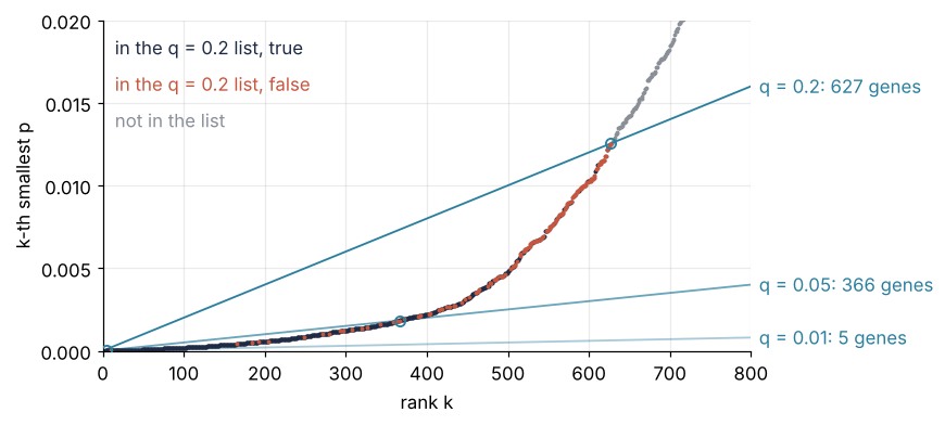
For the first 300 ranks the curve stays near zero, below p = 0.00125, and only 10 of those 300 genes are null. Then the responders thin out, the null genes take over, and past rank 650 the curve climbs as a straight line with close to the null slope of 1/9,500. The line at q = 0.01 crosses the curve at rank 5, at q = 0.05 at rank 366, and at q = 0.2 at rank 627. Inside the q = 0.2 list the red dots, null genes, gather where the curve bends upward.

Now let q run from 0.002 to 0.3 and watch the line and the list:

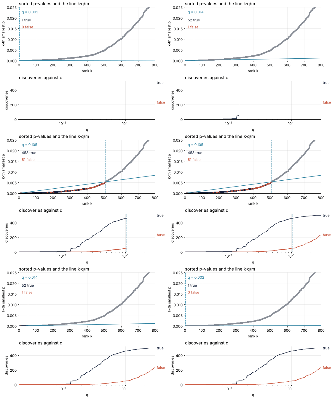
How I built this: each frame redraws the sorted p-values and the line for one q with Matplotlib's FuncAnimation, the technique of Matplotlib animation with FuncAnimation; the source is animations/bh-line/scene.py.

As q grows, the line tilts up and the cutoff jumps outward in steps. The false discoveries grow faster than the true ones, because the true ones run out. The share of false hits in the list is near zero while q is small and close to q from about q = 0.05 upward.

Formalization

Write m for the number of tests, m₀ for the number of true null hypotheses among them, R for the number of rejections (the hit list), and V for the false rejections in it. Here m = 10,000 and m₀ = 9,500, and R and V change from screen to screen. E[·] means the average over many repeats of the same screen.

The classical error rate is the family-wise error rate, FWER = P(V ≥ 1), the chance of at least one false hit. Uncorrected and for independent tests, it is 1 − 0.95^m₀: 64 % at m₀ = 20, and indistinguishable from 1 at 9,500. The union bound says that the chance of at least one of several events is never more than the sum of their chances. So m tests at α/m each give FWER ≤ m · α/m = α. The m₀ null genes among them give on average m₀·α/m false hits, which is at most α. That is the Bonferroni correction: test each gene at 0.05/10,000 = 5 × 10⁻⁶.

The false discovery rate asks a different question, how much of the list is wrong:

In words, it is the share of false hits in the list, averaged over screens, with an empty list counting as 0. The Benjamini-Hochberg rule sorts the p-values, \(p_{(1)} \le p_{(2)} \le \dots \le p_{(m)}\), finds

and rejects \(p_{(1)}, \dots, p_{(k)}\). Benjamini and Hochberg (1995) proved that for independent tests this keeps FDR ≤ q·m₀/m. Real genes are not independent: genes of one pathway rise and fall together, and so do their t-statistics. Benjamini and Yekutieli (2001) extended the proof to such positive correlation for one-sided tests, but two-sided tests like the ones here are not covered in general. They also gave a stricter variant that holds for any correlation. The rule is five lines of NumPy, SciPy has it as false_discovery_control since version 1.11, and the stricter variant is its option method="by":

q = 0.05
p_sorted = np.sort(p)
under = np.nonzero(p_sorted <= np.arange(1, M + 1) * q / M)[0]
k = under[-1] + 1                     # the largest rank under the line, not the first crossing
cutoff = p_sorted[k - 1]
by_hand = p <= cutoff

by_scipy = stats.false_discovery_control(p) <= q
print(f"by hand: {by_hand.sum()} discoveries   SciPy: {by_scipy.sum()}   "
      f"same genes: {np.array_equal(by_hand, by_scipy)}")
print(f"k = {k}   cutoff p_(k) = {cutoff:.5f}")
print(f"expected null genes below the cutoff: {(M - M1) * cutoff:.1f}   "
      f"observed: {by_hand[~responder].sum()}")
print(f"Bonferroni cutoff p = {0.05 / M:.0e} needs |t| > {stats.t.isf(0.05 / M / 2, df=2 * N - 2):.1f}")
print(f"same q, stricter routes: Welch's p-values {np.sum(stats.false_discovery_control(p_welch) <= q)} genes   "
      f"method='by' {np.sum(stats.false_discovery_control(p, method='by') <= q)} genes")

by hand: 366 discoveries   SciPy: 366   same genes: True
k = 366   cutoff p_(k) = 0.00183
expected null genes below the cutoff: 17.4   observed: 17
Bonferroni cutoff p = 5e-06 needs |t| > 33.0
same q, stricter routes: Welch's p-values 67 genes   method='by' 3 genes

Both find the same 366 genes, with the cutoff at p₍₃₆₆₎ = 0.00183. With Welch's p-values the same q gives 67 genes, the price of keeping Welch at three replicates. The stricter variant keeps 3, fewer even than Bonferroni: it divides q by 1 + 1/2 + … + 1/m, which is 9.8 here, so its line lies below Bonferroni's cutoff of 5 × 10⁻⁶ for the first nine ranks. So for correlated genes tested two-sided, which is the usual screen, the Benjamini-Hochberg q is covered by neither proof, and the variant that is covered leaves almost nothing. DESeq2 and limma report the Benjamini-Hochberg list all the same: read its q as a target, and confirm the hits you build on with a second experiment.

Why the line controls the false share. At a cutoff t, about m₀·t null genes fall below it, because their p-values are uniform. The rule picks t = k·q/m, where k is the number of discoveries. The expected false share is then m₀·t/k = q·m₀/m, which is at most q because m₀ is at most m. In this screen, 9,500 × 0.00183 gives 17.4 expected null genes among 366 discoveries, 4.7 %, and 17 are observed. This is the counting argument, not the proof; the paper has the proof.

What Bonferroni costs. A cutoff of 5 × 10⁻⁶ at 4 degrees of freedom (3 + 3 − 2 for Student's test) needs |t| > 33.0. A responder with a fourfold change reaches that only when its noise happens to be small, so 5 of the 500 survive in this screen. No false hit, and almost no true one either.

The FDR is an average over screens. It bounds E[V/R], not the share in any one list. Rerun the screen 200 times with the same truth and fresh noise:

rng_repeat = np.random.default_rng(1995)
false_share, bonferroni_true, raw_false = [], [], []
for _ in range(200):
    c, t = simulate_screen(rng_repeat)
    p_rep = stats.ttest_ind(t, c, axis=1).pvalue
    hits = stats.false_discovery_control(p_rep) <= q
    false_share.append(hits[~responder].sum() / max(hits.sum(), 1))
    bonferroni_true.append(np.sum(p_rep[responder] < 0.05 / M))
    raw_false.append(np.sum(p_rep[~responder] < 0.05))

false_share = np.array(false_share)
print(f"BH, false share:          mean {false_share.mean():.3f}   sd {false_share.std():.3f}   "
      f"range {false_share.min():.3f} to {false_share.max():.3f}   (q m0 / m = {q * (M - M1) / M:.4f})")
print(f"Bonferroni, true hits:    mean {np.mean(bonferroni_true):.2f}")
print(f"uncorrected, false hits:  mean {np.mean(raw_false):.1f}")

BH, false share:          mean 0.047   sd 0.012   range 0.021 to 0.076   (q m0 / m = 0.0475)
Bonferroni, true hits:    mean 3.77
uncorrected, false hits:  mean 471.9

The mean false share is 0.047, against the bound q·m₀/m = 0.0475, and one screen in 200 had as much as 7.6 %. A single list can be worse than q; the promise is about the average. Bonferroni keeps 3.8 true genes on average, and no correction lets through 472 false ones.

See it in code

In practice the whole analysis is two SciPy calls, ttest_ind along the replicate axis and false_discovery_control on the result:

Show code

Copy

res = stats.ttest_ind(treated, control, axis=1)       # one Student's t-test per gene, all at once
p_adj = stats.false_discovery_control(res.pvalue)     # Benjamini-Hochberg adjusted p-values

methods = {
    "no correction": res.pvalue < 0.05,
    "Bonferroni": res.pvalue < 0.05 / M,
    "BH, q = 0.05": p_adj <= 0.05,
}
print(f"{'method':15s} {'true':>5s} {'false':>6s} {'false share':>12s}")
for name, hit in methods.items():
    n_true, n_false = hit[responder].sum(), hit[~responder].sum()
    print(f"{name:15s} {n_true:5d} {n_false:6d} {n_false / max(hit.sum(), 1):11.1%}")
print(f"\ngenes with adjusted p <= 0.2: {np.sum(p_adj <= 0.2)}")

fig, (ax1, ax2) = plt.subplots(2, 1, figsize=(7, 5.4), height_ratios=[1.3, 1])
ax1.hist([res.pvalue[~responder], res.pvalue[responder]], bins=bins, stacked=True,
         color=[ACCENT, INK], alpha=0.85, lw=0)
ax1.axhline((M - M1) / 20, color=MUTED, lw=1, ls="--")
ax1.text(0.065, 800, "responders", color=INK, va="center")
ax1.text(0.99, 560, "null genes", ha="right", va="bottom", color=ACCENT)
ax1.set(xlabel="p-value", ylabel="genes per bin", xlim=(0, 1))
names = list(methods)[::-1]
n_true = np.array([methods[n][responder].sum() for n in names])
n_false = np.array([methods[n][~responder].sum() for n in names])
ax2.barh(names, n_true, color=INK, alpha=0.85, height=0.6)
ax2.barh(names, n_false, left=n_true, color=ACCENT, alpha=0.85, height=0.6)
for ax in (ax1, ax2):
    ax.set_axisbelow(True)                             # grid behind the bars
for y, (a, b) in enumerate(zip(n_true, n_false)):
    ax2.text(a + b + 15, y, f"{a} true, {b} false", va="center")
ax2.set(xlabel="discoveries", xlim=(0, 1300))
ax2.grid(axis="y", visible=False)
fig.tight_layout()
plt.show()

method           true  false  false share
no correction     500    488       49.4%
Bonferroni          5      0        0.0%
BH, q = 0.05      349     17        4.6%

genes with adjusted p <= 0.2: 627

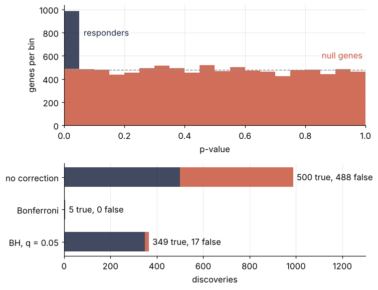
Compare with the truth. No correction finds all 500 responders and 488 null genes with them, a list that is half noise. Bonferroni finds 5 and no false one. Benjamini-Hochberg at q = 0.05 finds 349 of the 500 with 17 false, a false share of 4.6 % against the 5 % that was asked for.

false_discovery_control does not return a list. It returns one adjusted p-value per gene, the smallest q at which the rule would put that gene on the list. So "adjusted p ≤ 0.05" is the list at q = 0.05, and a gene with an adjusted p of 0.2 joins only if you accept a false share of 20 %; 627 genes qualify at that level. DESeq2 reports the same adjustment in its padj column, with one difference: it first sets aside genes with a low mean count or an outlier sample, gives them NA, and adjusts over the rest.

Where it shows up

Any field that runs one test per gene, voxel, mass bin, or trial frequency meets the 488 false genes of this screen in its own units, and has a name for its correction.

• Genomics and proteomics. RNA-seq tools report Benjamini-Hochberg adjusted p-values by default, in the padj column for DESeq2 and the adj.P.Val column for limma. Genome-wide association studies use p < 5 × 10⁻⁸, a Bonferroni cutoff for about a million independent variants across the genome.
• Neuroimaging. An fMRI contrast tests about 10⁵ voxels at once, so an uncorrected map at p < 0.05 lights up about 5,000 voxels where nothing happens. The field controls the family-wise error rate with random field theory or with permutation tests, two ways of accounting for neighboring voxels being correlated, and uses FDR as the less strict alternative.
• Particle physics. A bump hunt scans a range of masses for an excess, and a 3σ bump somewhere in a wide range is far more likely than at one mass fixed in advance. Physicists call this the look-elsewhere effect and quote local and global significance separately. It is one of the reasons for the 5σ convention of the 2012 Higgs discovery, which both experiments announced on local significance.
• Astronomy and gravitational waves. A periodogram of a star's radial velocity tests thousands of trial periods, so exoplanet searches report the false-alarm probability of the highest peak over all of them. Gravitational-wave detectors rank their candidates by a false-alarm rate, how often noise alone produces an event at least that loud.

In every case the threshold has to know how many places you looked.

Further reading

• The SciPy reference for scipy.stats.false_discovery_control and scipy.stats.ttest_ind.
• Benjamini and Hochberg, J. R. Stat. Soc. B 57, 289 (1995), the paper that introduced the rule and proves the bound, and Benjamini and Yekutieli, Ann. Stat. 29, 1165 (2001), for dependent tests.
• Efron, Large-Scale Inference (Cambridge, 2010), for thousands of tests at once as an empirical Bayes problem.
• Related tutorials on this site: scipy.stats from the ground up: is the difference between two samples real?, The standard error of the mean: why four times the data halves the error, Matplotlib animation with FuncAnimation: a probe sweep as a small GIF, HypothesisTests.jl from the ground up: do two samples really differ?, the same t-test in Julia, and this tutorial in Julia (planned).
• Download the notebook. It was executed with the library versions in the header.