PyBaMM from the ground up: a lithium-ion cell's capacity at fast discharge

The problem: how much charge does a fast discharge leave behind?

The LG M50 is a cylindrical lithium-ion cell rated at 5 A h. A current that would empty that rating in one hour is called 1C, so for this cell 2C is 10 A and C/10 is 0.5 A. PyBaMM, an open-source package of battery models, ships a parameter set for the M50, and its model says: drawn at C/10 the cell delivers 5.08 A h before the voltage reaches the 2.5 V cutoff. At 2C it stops after 28.4 minutes with 4.73 A h, at 3C with 2.30 A h, less than half.

Each electrode is a porous layer of micrometer-sized particles that store lithium in their crystal lattice, soaked in electrolyte. The stack is negative electrode, separator, positive electrode, 173 µm in all. On discharge, lithium leaves the negative particles, crosses the electrolyte as ions, and enters the positive particles. The Doyle-Fuller-Newman model (DFN) describes this as two diffusion problems, ions across the stack and lithium along the radius of every particle, coupled at the particle surfaces: the kind of problem you met in the heat equation on a grid.

The cell voltage is the difference of the two electrodes' potentials, and each is set by the lithium content at its particle surfaces, through an open-circuit curve that plays the role of the Nernst equation and turns steep near empty and near full. A fast discharge drains a surface faster than diffusion refills it from inside. And where the electrolyte runs out of ions, the particles behind that spot react only at a large extra voltage. Either way the voltage hits 2.5 V before the lithium is used up. So what ends the 2C run early, the electrolyte or the particles?

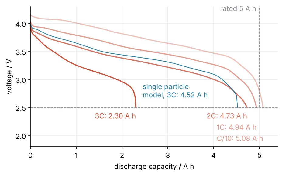
Cell voltage against delivered charge for discharges at C/10, 1C, 2C, and 3C, from the Doyle-Fuller-Newman model. The capacity at the 2.5 V cutoff falls from 5.08 to 2.30 A h. A thin blue line, the single particle model at 3C, reaches 4.52 A h.

This is where we end up: the same cell discharged at four rates, the delivered charge falling slowly up to 2C and collapsing at 3C, and a simpler model that misses the collapse; the dashed lines mark the cutoff and the rating. Step 6 draws it.

Setup

Install the library with pip install pybamm. The first line opts out of PyBaMM's usage telemetry; without it, the first import asks for consent and waits 10 s for an answer.

import os
os.environ["PYBAMM_DISABLE_TELEMETRY"] = "true"
import warnings
warnings.filterwarnings("ignore", message="IProgress not found")   # tqdm, harmless without ipywidgets

import numpy as np
import matplotlib.pyplot as plt
import pybamm

plt.rcParams.update({
    "figure.figsize": (7, 4), "figure.dpi": 110,
    "axes.spines.top": False, "axes.spines.right": False,
    "axes.grid": True, "grid.alpha": 0.25,
    "font.size": 11, "lines.linewidth": 1.8,
})
INK, ACCENT, SECOND, MUTED = "#1f2a44", "#c8553d", "#2a7f9e", "#8a8f98"

print("PyBaMM", pybamm.__version__)

PyBaMM 26.10.0.0

Step 1: Run a model with its defaults

A PyBaMM run takes three objects: a model, which holds the equations, a simulation, which discretizes them and calls a solver, and the solution that comes back. The simulation fills in a default parameter set, grid, and solver, so the shortest run is three lines:

model = pybamm.lithium_ion.DFN()
sim = pybamm.Simulation(model)
sol = sim.solve([0, 3600])    # time span in seconds

built = sim.built_model
print(model.name)
print("termination:  ", sol.termination)
print(f"final voltage: {sol['Voltage [V]'].entries[-1]:.2f} V")
print("unknowns:      ", built.concatenated_rhs.size, "differential,",
      built.concatenated_algebraic.size, "algebraic")
print(f"capacity of the default cell: {sim.parameter_values['Nominal cell capacity [A.h]']:.2f} A h")

Doyle-Fuller-Newman model
termination:   final time
final voltage: 3.17 V
unknowns:       862 differential, 100 algebraic
capacity of the default cell: 0.68 A h

The run went for the hour it was asked for and ended at 3.17 V. Of the 862 differential unknowns, 860 are the lithium concentrations on PyBaMM's grid, 20 cells in each of the three regions of the stack and 20 along the radius of a particle in each electrode cell, every one an ODE in time, as in the method of lines; the other two are counters of the delivered charge. The 100 algebraic ones are the electric potentials in the electrolyte and in the two electrodes. They have no time derivative: at every instant the condition that the same current flows through every slice of the stack fixes them. A system of ODEs plus equations without a derivative is a differential-algebraic equation (DAE), and PyBaMM picks a solver that handles one.

The last line is the catch. The default set takes the per-area properties of a graphite and lithium cobalt oxide cell from Marquis et al. (2019) and puts them on one electrode sheet of 13.7 cm by 20.7 cm, which makes 0.68 A h. It is not the M50. The defaults are a demonstration, not your cell.

Step 2: Choose a parameter set and change a value in it

A parameter set is a dictionary from names to values. Chen2020 is the M50:

param = pybamm.ParameterValues("Chen2020")
for name in ["Nominal cell capacity [A.h]", "Lower voltage cut-off [V]",
             "Upper voltage cut-off [V]", "Current function [A]"]:
    print(f"{name:30s} {param[name]}")
print()

param.search("diffusivity", print_values=False)
for name in ["Negative particle diffusivity [m2.s-1]", "Positive particle diffusivity [m2.s-1]",
             "Electrolyte diffusivity [m2.s-1]"]:
    value = param[name]
    print(f"{name:40s} {value.__name__ if callable(value) else value}")

Nominal cell capacity [A.h]    5.0
Lower voltage cut-off [V]      2.5
Upper voltage cut-off [V]      4.2
Current function [A]           5.0

Results for 'diffusivity': ['SEI solvent diffusivity [m2.s-1]', 'SEI lithium interstitial diffusivity [m2.s-1]', 'EC diffusivity [m2.s-1]', 'Negative particle diffusivity [m2.s-1]', 'Positive particle diffusivity [m2.s-1]', 'Electrolyte diffusivity [m2.s-1]']
Negative particle diffusivity [m2.s-1]   3.3e-14
Positive particle diffusivity [m2.s-1]   4e-15
Electrolyte diffusivity [m2.s-1]         electrolyte_diffusivity_Nyman2008

The capacity is 5.0 A h, the voltage window 2.5 V to 4.2 V, and the current of a plain solve 5 A. search finds every name containing a word, which is how you learn the names: they are long strings with the unit in brackets, and they must be typed exactly. The particle diffusivities are plain numbers, 3.3e-14 m²/s in the negative electrode and eight times smaller in the positive one. The electrolyte diffusivity is a Python function, electrolyte_diffusivity_Nyman2008, that takes the concentration and the temperature and uses only the concentration.

To change a value, copy the set and assign to the copy, by item or with update for several at once:

p = param.copy()
p.update({"Negative particle diffusivity [m2.s-1]": 3.3e-13})
print(p["Negative particle diffusivity [m2.s-1]"], param["Negative particle diffusivity [m2.s-1]"])

3.3e-13 3.3e-14

The original is untouched. A function-valued parameter is replaced by another function with the same arguments, here (c_e, T). Step 5 does both.

Step 3: Describe the discharge as an experiment

sim.solve([0, 3600]) runs for a fixed time at a fixed current. What you want from a cell is usually a protocol: discharge at some rate until some voltage. PyBaMM reads that from a string:

model = pybamm.lithium_ion.DFN()
experiment = pybamm.Experiment(["Discharge at 2C until 2.5 V"])
sim = pybamm.Simulation(model, parameter_values=param, experiment=experiment)
sol = sim.solve()

V = sol["Voltage [V]"].entries
Q = sol["Discharge capacity [A.h]"].entries
print("termination:", sol.termination)
print(f"time to cutoff {sol['Time [min]'].entries[-1]:.1f} min, delivered {Q[-1]:.2f} A h")
print("voltage at", ", ".join(f"{q} A h: {np.interp(q, Q, V):.2f} V" for q in (3.5, 4.0, 4.3)))

termination: event: Voltage < 2.5 [V] [experiment]
time to cutoff 28.4 min, delivered 4.73 A h
voltage at 3.5 A h: 3.13 V, 4.0 A h: 3.00 V, 4.3 A h: 2.88 V

The run ended on the voltage event after 28.4 minutes, with 4.73 A h delivered. "2C" is read against the parameter set's nominal capacity, so this is 10 A; "Discharge at 10 A until 2.5 V" is the same experiment. The same string language has rests, charges, constant-voltage holds, and repeated cycles.

fig, ax = plt.subplots(figsize=(7, 3.6))
ax.plot(Q, V, color=ACCENT)
ax.axhline(2.5, color=MUTED, lw=1, ls="--")
ax.text(0.1, 2.55, "2.5 V cutoff", color=MUTED)
ax.set(xlabel="discharge capacity / A h", ylabel="voltage / V", xlim=(0, 5.2))
plt.show()

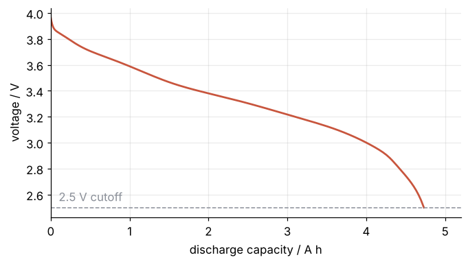
Cell voltage in V against delivered charge in A h for a 2C discharge of the M50. The voltage falls slowly from about 3.9 V, then drops steeply in the last few percent to the 2.5 V cutoff at 4.73 A h.

The voltage slides down gently for most of the discharge and then bends sharply: it loses 0.13 V from 3.5 to 4.0 A h and 0.38 V over the last 0.43 A h. By the voltage link of the motivation, that knee means some particle surface or some stretch of electrolyte has reached its limit.

Step 4: Read voltage and concentrations from the solution

In the solution, x runs across the stack in meters, from the negative current collector (the metal foil that carries the current out of the negative electrode) to the positive one, and r runs inside a particle. The lithium content of a particle is given as stoichiometry, the fraction of the most it can hold: 0 is empty, 1 is full. On discharge the negative particles go toward 0 and the positive ones toward 1.

Indexing the solution by a variable name returns a processed variable. Its .entries is a NumPy array with time as the last axis, and calling it with t= in seconds (and x= in meters) interpolates:

c_e = sol["Electrolyte concentration [mol.m-3]"]
x = sol["x [m]"].entries[:, 0]
sto_n = sol["Negative particle surface stoichiometry"]
sto_p = sol["Positive particle surface stoichiometry"]
print("shapes:", c_e.entries.shape, x.shape, sto_n.entries.shape, sto_p.entries.shape)

L_n, L_s, L_p = (param[f"{d} thickness [m]"] for d in ["Negative electrode", "Separator", "Positive electrode"])
print(f"negative {L_n*1e6:.1f} µm, separator {L_s*1e6:.1f} µm, positive {L_p*1e6:.1f} µm")

print(f"electrolyte at the end: {c_e.entries[0, -1]:5.0f} mol/m³ by the negative collector, "
      f"{c_e.entries[-1, -1]:3.0f} by the positive one (start {c_e.entries[0, 0]:.0f})")
print(f"negative surface stoichiometry {sto_n.entries[:, -1].min():.2f} to {sto_n.entries[:, -1].max():.2f}, "
      f"particle average {sol['Average negative particle stoichiometry'].entries[-1]:.2f}")
print(f"positive surface stoichiometry {sto_p.entries[:, -1].min():.2f} to {sto_p.entries[:, -1].max():.3f}, "
      f"particle average {sol['Average positive particle stoichiometry'].entries[-1]:.2f}")
U_n = sol["X-averaged negative electrode open-circuit potential [V]"].entries
print(f"negative open-circuit potential {U_n[0]:.2f} V at the start, {U_n[-1]:.2f} V at the end")

shapes: (60, 180) (60,) (20, 180) (20, 180)
negative 85.2 µm, separator 12.0 µm, positive 75.6 µm
electrolyte at the end:  3325 mol/m³ by the negative collector,  67 by the positive one (start 1000)
negative surface stoichiometry 0.05 to 0.06, particle average 0.09
positive surface stoichiometry 0.91 to 0.998, particle average 0.81
negative open-circuit potential 0.09 V at the start, 0.62 V at the end

The electrolyte has 60 cells across the stack, each surface stoichiometry 20 cells across its electrode. By the end the electrolyte has piled up to 3,325 mol/m³ by the negative collector and fallen from 1,000 to 67 by the positive one. The negative particle surfaces are nearly empty, 0.05 against an average of 0.09 inside. The positive surfaces reach 0.998 against an average of 0.81. The last line ties a concentration to the voltage: the negative electrode's open-circuit potential climbs from 0.09 V to 0.62 V, and every volt it gains is a volt the cell loses.

t_min = [0, 10, 20, sol["Time [min]"].entries[-1]]
alphas = [0.35, 0.55, 0.8, 1.0]
um = 1e6

fig, (ax1, ax2) = plt.subplots(2, 1, figsize=(7, 4.4), sharex=True)
for t, a in zip(t_min, alphas):
    ts = 60 * t
    ax1.plot(x * um, c_e(t=ts), color=ACCENT, alpha=a)
    ax2.plot(sol["x_n [m]"].entries[:, 0] * um, sto_n(t=ts), color=ACCENT, alpha=a)
    ax2.plot(sol["x_p [m]"].entries[:, 0] * um, sto_p(t=ts), color=ACCENT, alpha=a)
    ax2.text(4, sto_n(t=ts)[0] + 0.03, f"{t:.0f} min", color=ACCENT, alpha=max(a, 0.6), va="bottom")
for b in (L_n, L_n + L_s):                       # electrode boundaries, kept below the region labels
    ax1.axvline(b * um, ymax=0.84, color=MUTED, lw=1, ls="--")
    ax2.axvline(b * um, color=MUTED, lw=1, ls="--")
ax2.hlines(0, 0, L_n * um, color=MUTED, lw=1, ls="--")                       # empty, where the negative heads
ax2.hlines(1, (L_n + L_s) * um, (L_n + L_s + L_p) * um, color=MUTED, lw=1, ls="--")   # full, the positive
for xc, label in [(L_n / 2, "negative"), (L_n + L_s / 2, "separator"), (L_n + L_s + L_p / 2, "positive")]:
    ax1.text(xc * um, 3650, label, color=INK, ha="center")
ax1.set(ylabel="electrolyte / mol m⁻³", ylim=(0, 4000))
ax2.set(xlabel="position across the cell x / µm", ylabel="surface stoichiometry", ylim=(-0.05, 1.1))
plt.show()

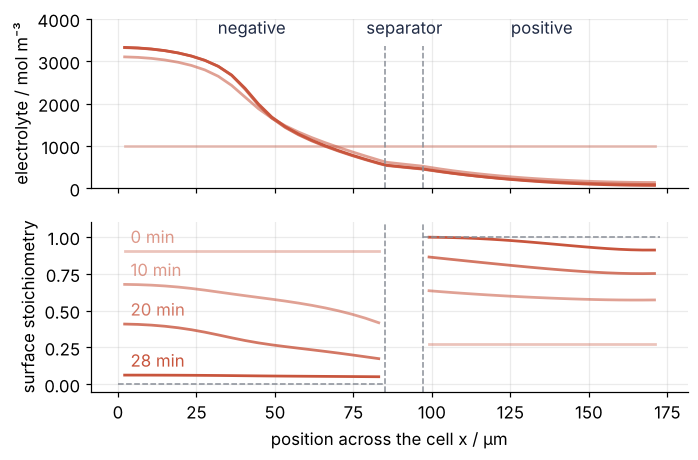
Two panels across the cell, position in µm. Top: electrolyte concentration at 0, 10, 20 minutes and the end of a 2C discharge, rising on the negative side and falling to near zero at the positive end. Bottom: particle surface stoichiometry, the negative surfaces sinking toward 0 and the positive ones rising toward 1.

Everything moves toward a limit at once: the negative surfaces toward empty, the positive surfaces toward full next to the separator, the electrolyte thinning at the far end. The picture cannot say which of these costs the missing charge.

Step 5: Change one value to find the bottleneck

Make each process ten times faster in a copy of the parameter set, run the same discharge, and see which gives back the missing charge. The factor is equal for both, so neither gets an advantage, and it is large, so the answer does not hide in the second decimal. period sets only how often the solution is recorded, not its accuracy:

def capacity(p, c_rate, model=model):
    experiment = pybamm.Experiment([f"Discharge at {c_rate}C until 2.5 V"], period="10 seconds")
    sol = pybamm.Simulation(model, parameter_values=p, experiment=experiment).solve()
    return sol["Discharge capacity [A.h]"].entries[-1], sol

fast_particles = param.copy()
for name in ["Negative particle diffusivity [m2.s-1]", "Positive particle diffusivity [m2.s-1]"]:
    fast_particles[name] = 10 * param[name]

D_e = param["Electrolyte diffusivity [m2.s-1]"]
fast_electrolyte = param.copy()
fast_electrolyte["Electrolyte diffusivity [m2.s-1]"] = lambda c_e, T: 10 * D_e(c_e, T)

print("C-rate   baseline   particles x10   electrolyte x10   (A h)")
for c_rate in [2, 3]:
    q = [capacity(p, c_rate)[0] for p in (param, fast_particles, fast_electrolyte)]
    print(f"{c_rate}C       {q[0]:5.2f}       {q[1]:5.2f}           {q[2]:5.2f}")

split = []
for name in ["Negative particle diffusivity [m2.s-1]", "Positive particle diffusivity [m2.s-1]"]:
    p = param.copy()
    p[name] = 10 * param[name]
    split.append(capacity(p, 2)[0])
print(f"2C with only the negative particles x10: {split[0]:.2f} A h, only the positive: {split[1]:.2f} A h")

for c_rate in [2, 3]:
    s = capacity(param, c_rate)[1]
    c_end = max(s["Electrolyte concentration [mol.m-3]"].entries[-1, -1], 0.0)   # the solver can return a tiny negative number
    eta = -s["Positive electrode reaction overpotential [V]"].entries[-1, -1]
    print(f"{c_rate}C at the cutoff, by the positive collector: electrolyte {c_end:3.0f} mol/m³, "
          f"extra voltage of the reaction {eta:.2f} V; "
          f"average negative stoichiometry {s['Average negative particle stoichiometry'].entries[-1]:.2f}")

C-rate   baseline   particles x10   electrolyte x10   (A h)
2C        4.73        4.97            4.80
3C        2.30        3.30            4.52
2C with only the negative particles x10: 4.87 A h, only the positive: 4.80 A h
2C at the cutoff, by the positive collector: electrolyte  67 mol/m³, extra voltage of the reaction 0.10 V; average negative stoichiometry 0.09
3C at the cutoff, by the positive collector: electrolyte   0 mol/m³, extra voltage of the reaction 0.91 V; average negative stoichiometry 0.51

At 2C faster particles give back 4.97 A h, more than the 4.94 A h of the 1C run, while a faster electrolyte gains only 0.07 A h. Most of the particle gain comes from the negative ones, whose surfaces Step 4 found nearly empty: speeding up only them gives 4.87 A h, only the positive ones 4.80. The answer to the opening question is the negative particles.

The 67 mol/m³ left by the positive collector does not end the 2C run, because in Chen2020 the reaction rate goes with the square root of the electrolyte concentration. At 67 instead of 1,000 it drops to a quarter, and the reaction there needs 0.10 V extra, small next to the 0.53 V the negative open-circuit potential climbed. At 3C the order flips. A faster electrolyte brings the capacity from 2.30 to 4.52 A h, faster particles only to 3.30. The electrolyte by the positive collector is empty at the cutoff, the square root is zero, and the reaction there needs 0.91 V extra while the negative particles are still half full. That extra voltage, not an open-circuit curve, takes the cell to 2.5 V. This is an experiment on the model, not a recipe for a better cell.

Step 6: Sweep the C-rate and compare with the single particle model

The single particle model (SPM) keeps one particle per electrode and assumes the electrolyte carries any current without its concentration changing. Build each model once and pass it to a new simulation per rate; build discretizes a model without solving it, which is enough to count its unknowns:

c_rates = [0.1, 1, 2, 3]
models = {"DFN": pybamm.lithium_ion.DFN(), "SPM": pybamm.lithium_ion.SPM()}
spm_sim = pybamm.Simulation(models["SPM"], parameter_values=param)
spm_sim.build()                                  # discretize without solving, to count
print("SPM unknowns:", spm_sim.built_model.concatenated_rhs.size, "differential,",
      spm_sim.built_model.concatenated_algebraic.size, "algebraic\n")

curves = {}
for name, m in models.items():
    for c_rate in c_rates:
        q, s = capacity(param, c_rate, model=m)
        curves[name, c_rate] = (s["Discharge capacity [A.h]"].entries, s["Voltage [V]"].entries)

print("C-rate    DFN     SPM   (A h)")
for c_rate in c_rates:
    print(f"{c_rate:4g}C   {curves['DFN', c_rate][0][-1]:5.2f}   {curves['SPM', c_rate][0][-1]:5.2f}")

labels = {0.1: "C/10", 1: "1C", 2: "2C", 3: "3C"}
fig, ax = plt.subplots()
for c_rate, a in zip(c_rates, [0.35, 0.55, 0.8, 1.0]):
    Q, V = curves["DFN", c_rate]
    ax.plot(Q, V, color=ACCENT, alpha=a)
    y_label = {0.1: 1.95, 1: 2.15, 2: 2.35, 3: 2.35}[c_rate]
    ax.text(Q[-1], y_label, f"{labels[c_rate]}: {Q[-1]:.2f} A h", color=ACCENT, alpha=max(a, 0.6),
            ha="right", va="center")
Q, V = curves["SPM", 3]
ax.plot(Q, V, color=SECOND, lw=1.1)
ax.text(2.45, 2.8, f"single particle\nmodel, 3C: {Q[-1]:.2f} A h", color=SECOND, va="center")
ax.axhline(2.5, color=MUTED, lw=1, ls="--")
ax.plot([5.0, 5.0], [2.5, 4.3], color=MUTED, lw=1, ls="--")
ax.text(4.93, 4.22, "rated 5 A h", color=MUTED, ha="right")
ax.set(xlabel="discharge capacity / A h", ylabel="voltage / V", xlim=(0, 5.4), ylim=(1.8, 4.3))
plt.show()

SPM unknowns: 42 differential, 0 algebraic

C-rate    DFN     SPM   (A h)
 0.1C    5.08    5.08
   1C    4.94    4.96
   2C    4.73    4.82
   3C    2.30    4.52

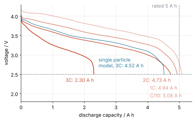
Cell voltage in V against delivered charge in A h at C/10, 1C, 2C, and 3C from the Doyle-Fuller-Newman model, darker for faster rates, with the capacities at the 2.5 V cutoff labeled. A thin blue line, the single particle model at 3C, reaches 4.52 A h where the full model stops at 2.30 A h.

The SPM has 42 unknowns where the DFN has 962. Up to 2C, where the particles limit, the SPM stays within 2 % of the DFN. At 3C, where the electrolyte limits, it gives 4.52 A h against 2.30, twice the full model and the same number Step 5 got from the DFN with a ten times faster electrolyte. The SPM is the DFN with a perfect electrolyte, and it cannot see the electrolyte run dry. A model that leaves out the process that limits you will not show you the limit, so check the fastest rate you care about with the DFN. The 3C numbers are what the model predicts, not a measurement on a real M50.

Pitfalls

A misspelled parameter name. Assigning to a name that does not exist raises nothing; it adds a new key that no equation reads:

p = param.copy()
p.update({"Negative particle diffusivty [m2.s-1]": 3.3e-13})   # "diffusivty"
print(f"2C with the 'faster' particles: {capacity(p, 2)[0]:.2f} A h")
try:
    param["Negative particle diffusivty [m2.s-1]"]
except KeyError as err:
    print("reading it: KeyError, best matches", err.args[0].split("Best matches are ")[1])

2C with the 'faster' particles: 4.73 A h
reading it: KeyError, best matches ['Negative particle diffusivity [m2.s-1]', 'Positive particle diffusivity [m2.s-1]', 'Negative particle radius [m]']

The run gives 4.73 A h, as if nothing had changed, because nothing had. Reading the misspelled name does fail, with a list of close matches. Find names with param.search(...) and check name in param.keys() before you update.

A run that stops early without saying so. Set Current function [A] to 10 in a copy of the set and call solve([0, 3600]): the run ends before the hour is up, on the minimum-voltage event, and nothing warns you. Arrays are shorter than you expect and the plot ends early. The termination message from Steps 1 and 3 says so, and so does sol.t[-1] compared with the time span you asked for. When the cutoff is the point, use an experiment.

Reading a particle array in the wrong axis order. sol["Positive particle stoichiometry"].entries has shape (radius, position, time), 20 × 20 × 180 for the 2C solution of Steps 3 and 4. entries[:, :, -1] is the last time; entries[-1] is the outermost radial cell at every position and every time, which plots as nonsense with plausible numbers. Call the variable with t=, x=, and r= in meters instead, and check the radial grid against sol["r_p [m]"].

Variations

A drive cycle. Replace the string by pybamm.step.current(data) inside the Experiment, with data a two-column array of time and current.
A cell that heats up. pybamm.lithium_ion.DFN(options={"thermal": "lumped"}) adds a temperature. Of the parameter functions in Chen2020, only the two exchange current densities depend on it.
Capacity fade over cycles. options={"SEI": "solvent-diffusion limited"} and an experiment of discharge, rest, charge, and hold, repeated with [(...)] * N; sol.summary_variables holds the capacity per cycle.
Another chemistry. Load another of PyBaMM's parameter sets, for instance the LFP cell Prada2013, and rerun the same three lines.

Cheat sheet

model = pybamm.lithium_ion.DFN()                       # or SPM(): uniform electrolyte, wrong when it limits
param = pybamm.ParameterValues("Chen2020")             # the defaults are a demo cell, not yours
param.search("diffusivity")                            # names are exact strings with units
p = param.copy(); p.update({name: value})              # misspelled names are silently added
exp = pybamm.Experiment(["Discharge at 2C until 2.5 V"])
sol = pybamm.Simulation(model, parameter_values=p, experiment=exp).solve()
sol.termination                                        # why it stopped
sol["Voltage [V]"].entries                             # NumPy array, time on the last axis
sol["Discharge capacity [A.h]"].entries[-1]            # delivered charge
sol["Electrolyte concentration [mol.m-3]"](t=600, x=1e-4)  # interpolate, SI units