Finite volumes: why a conservation law is solved by bookkeeping the fluxes

The question

A pipe 2 m long carries water at 5 cm/s. Between 0.8 m and 1.2 m it narrows like a Venturi tube, abruptly on the way in and gradually on the way out, and in the throat the water runs 3.67 times faster. A Gaussian pulse of dye with a standard deviation of 2.5 cm starts at 0.40 m and is carried through. Describe it by \(c(x, t)\), the amount of dye per meter of pipe, and treat the flow as one-dimensional plug flow without diffusion; a probe that reads concentration would see \(c\) divided by the cross-section.

Where the water speeds up, every slice of it is drawn out, and the curve of \(c\) drops with it: 8.5 s in, the pulse is 3.6 times as long as at the start and its peak is down to 0.32 of its initial height. No dye is lost. The same dye is spread over a longer stretch of pipe, and the area under the curve, the amount of dye, stays what it was. The law that says so is

with \(u(x)\) the speed of the water. The obvious way to compute it expands the derivative by the product rule, \(\partial c/\partial t = -u\,\partial c/\partial x - c\,du/dx\), takes \(du/dx\) from the formula for the pipe, and replaces \(\partial c/\partial x\) at each grid point by a central difference: the slope from the two neighbors, \((c_{i+1} - c_{i-1})/(2\Delta x)\). Here it is on 400 points 5 mm apart, with the exact pulse from following each slice of water:

Show code

Copy

import numpy as np
import matplotlib.pyplot as plt

plt.rcParams.update({
    "figure.figsize": (7, 3.6), "figure.dpi": 110,
    "axes.spines.top": False, "axes.spines.right": False,
    "axes.grid": True, "grid.alpha": 0.25,
    "font.size": 11, "lines.linewidth": 1.8,
})
INK, ACCENT, SECOND, MUTED = "#1f2a44", "#c8553d", "#2a7f9e", "#8a8f98"

# ---- the pipe: 2 m in 400 cells of 5 mm, a Venturi throat between 0.8 and 1.2 m
L, N, u0 = 2.0, 400, 0.05                          # m, cells, m/s in the wide pipe
dx = L / N
x = (np.arange(N) + 0.5) * dx                      # cell centers
x_face = np.arange(N + 1) * dx                     # faces, both pipe ends included

def area(x):
    """Cross-section relative to the wide pipe: abrupt entry, gradual exit."""
    return 1 - 0.375 * (np.tanh((x - 0.80) / 0.02) - np.tanh((x - 1.00) / 0.08))

def speed(x):
    return u0 / area(x)                            # the same volume of water per second through every section

def dudx(x):
    sech2 = lambda z: 1 / np.cosh(z)**2
    dA = -0.375 * (sech2((x - 0.80) / 0.02) / 0.02 - sech2((x - 1.00) / 0.08) / 0.08)
    return -u0 * dA / area(x)**2

# ---- the pulse, and the exact solution from following each slice of water
sigma0, x0 = 0.025, 0.40                           # m
def pulse(x):
    return np.exp(-0.5 * ((x - x0) / sigma0)**2)

x_fine = np.linspace(0, L, 400_001)
inv_u = 1 / speed(x_fine)
tau = np.concatenate([[0], np.cumsum(0.5 * (inv_u[1:] + inv_u[:-1]) * np.diff(x_fine))])   # travel time from x = 0

def exact(x, t):
    """The water now at x was at xi a time t ago, and the flux u*c it carries has not changed."""
    xi = np.interp(np.interp(x, x_fine, tau) - t, tau, x_fine, left=-1.0)
    return speed(xi) * pulse(xi) / speed(x)

# ---- time steps: Courant number 0.5 where the water is fastest
u_max = speed(x_fine).max()
t_end = 16.0                                       # s: past the throat, and no dye at the outlet yet
n_steps = int(np.ceil(t_end / (0.5 * dx / u_max)))
dt = t_end / n_steps
t_steps = np.arange(n_steps + 1) * dt

def rk3_step(c, rate, dt=dt):
    """Three-stage Runge-Kutta of Shu and Osher: a weighted average of forward Euler stages."""
    c1 = c + dt * rate(c)
    c2 = 0.75 * c + 0.25 * (c1 + dt * rate(c1))
    return c / 3 + 2 / 3 * (c2 + dt * rate(c2))

def run(rate, keep=()):
    """Advance the pulse to t_end; return the final c, the amount after every step, and snapshots."""
    c = pulse(x)
    amount, snaps = [c.sum() * dx], {}
    for n in range(1, n_steps + 1):
        c = rk3_step(c, rate)
        amount.append(c.sum() * dx)
        if n in keep:
            snaps[n] = c
    return c, np.array(amount), snaps

# ---- the obvious discretization: product rule, central difference for dc/dx, du/dx from the formula
u, du = speed(x), dudx(x)
def point_rate(c):
    cp = np.pad(c, 1)                              # clean water beyond both ends
    return -u * (cp[2:] - cp[:-2]) / (2 * dx) - c * du

c_point, amount_point, _ = run(point_rate)
drift_point = 100 * (amount_point / amount_point[0] - 1)
t_throat = [np.interp(xb, x_fine, tau) - np.interp(x0, x_fine, tau) for xb in (0.80, 1.20)]

print(f"fastest water   {u_max:.3f} m/s, {u_max / u0:.2f} times the wide pipe")
print(f"time step       {1e3 * dt:.1f} ms, {n_steps} steps to {t_end:.0f} s")
print(f"amount of dye   {drift_point.max():+.2f} % at t = {t_steps[drift_point.argmax()]:.1f} s, "
      f"{drift_point[-1]:+.2f} % at the end")

def half_width(t):
    c_t = exact(x_fine, t)
    return np.ptp(x_fine[c_t >= c_t.max() / 2])
print(f"exact pulse     peak {exact(x_fine, 8.5).max():.2f} at 8.5 s, in the throat; "
      f"{half_width(8.5) / half_width(0):.1f} times as long as at the start")

fig, (ax1, ax2) = plt.subplots(2, 1, figsize=(7, 5), layout="constrained")
ax1.axvspan(0.80, 1.20, color=MUTED, alpha=0.15, lw=0)
ax1.text(1.0, 1.08, f"throat, {u_max / u0:.1f}× faster", ha="center", color=MUTED)
for t in (0, 8.5, 16):
    ct = exact(x, t)
    ax1.plot(x, ct, color=INK)
    ax1.text(x[ct.argmax()], ct.max() + 0.04, f"{t:g} s", ha="center", va="bottom")
ax1.set(xlabel="x / m", ylabel="c / initial peak", xlim=(0.2, 1.7), ylim=(-0.05, 1.2))
ax2.axvspan(*t_throat, color=MUTED, alpha=0.15, lw=0)
ax2.text(np.mean(t_throat), 0.15, "pulse in throat", ha="center", va="center", color=MUTED)
ax2.axhline(0, color=MUTED, lw=1, ls="--")
ax2.plot(t_steps, drift_point, color=ACCENT)
i_peak = drift_point.argmax()
ax2.annotate(f"{drift_point[i_peak]:+.2f} %", (t_steps[i_peak], drift_point[i_peak]), xytext=(0, 4),
             textcoords="offset points", ha="center", va="bottom", color=ACCENT)
ax2.annotate(f"point by point, {drift_point[-1]:+.2f} %", (t_end, drift_point[-1]), xytext=(0, -8),
             textcoords="offset points", ha="right", va="top", color=ACCENT)
ax2.set(xlabel="t / s", ylabel="amount change / %", xlim=(0, t_end), ylim=(-0.03, 0.48))
plt.show()

fastest water   0.184 m/s, 3.67 times the wide pipe
time step       13.6 ms, 1176 steps to 16 s
amount of dye   +0.40 % at t = 8.2 s, +0.30 % at the end
exact pulse     peak 0.32 at 8.5 s, in the throat; 3.6 times as long as at the start

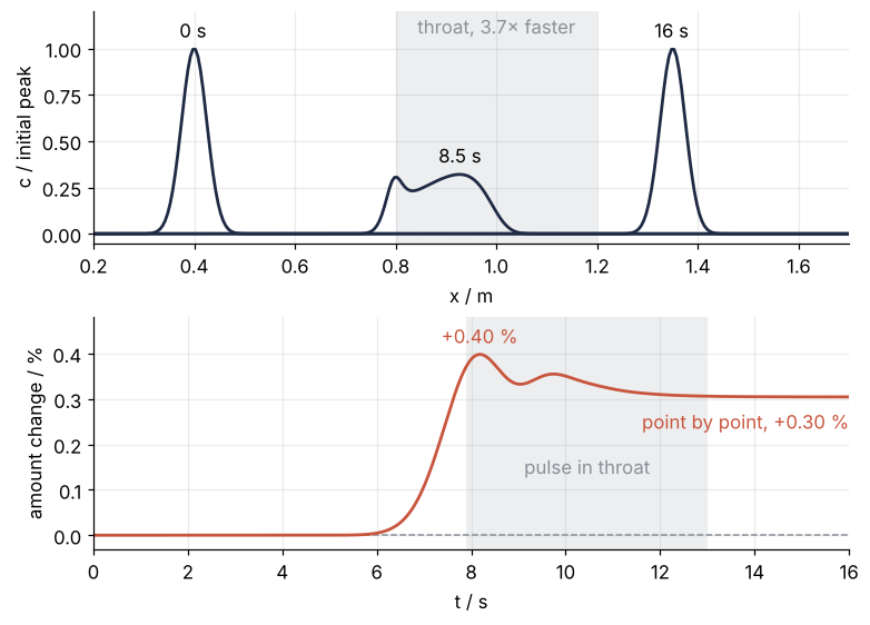
The pulse looks right: low and long in the throat, its old shape back after it. The scheme is also second order, which means that halving \(\Delta x\) quarters the error. But no dye enters or leaves this pipe, and the computed amount rises by 0.40 % as the pulse enters the throat and stays 0.30 % high after it has left.

So where does the dye come from that nobody added? And is there a way to discretize the law so that the amount cannot change, on any grid?

The idea: cells that trade dye through their faces

Cut the pipe into 400 cells of 5 mm, and for each cell keep the amount of dye it holds instead of a value at a point. The array stores that amount divided by \(\Delta x\), so it reads in the same units as \(c\). During a time step, dye crosses each face at the rate \(uc\) taken at that face. Subtract it from the cell it leaves and add it to the cell it enters.

Every transfer is entered twice, once with each sign, so the books balance by construction. The total can change only through the two ends of the pipe, and there is no dye there. This bookkeeping is the finite volume method, and the cells are its volumes.

One thing is missing. The cells hold averages, so \(c\) at a face is not known and has to be built from the two cells beside it. There are two simple choices: the mean of the two, called central, or the value of the cell the water comes from, called upwind. Whichever you pick, the bookkeeping is the same, and the total is kept either way. The function below returns each cell's flux in minus flux out, divided by \(\Delta x\), and the run advances it with the same time stepping as the point-by-point run (the Formalization says which). Central goes first, and the run keeps the cells at 7.5 s for a closer look:

u_face = speed(x_face)

def flux_rate(c, face):
    cp = np.pad(c, 1)                              # clean water beyond both ends
    left, right = cp[:-1], cp[1:]                  # the two cells beside each face
    if face == "central":
        c_face = 0.5 * (left + right)
    else:                                          # upwind: the cell the water comes from
        c_face = np.where(u_face > 0, left, right)
    F = u_face * c_face                            # dye per second through each face
    return (F[:-1] - F[1:]) / dx                   # in through the left face, out through the right

n_snap = round(7.5 / dt)
c_central, amount_central, snaps = run(lambda c: flux_rate(c, "central"), keep={n_snap})
print(f"amount change, point by point:           {amount_point[-1] / amount_point[0] - 1:+.1e}")
print(f"amount change, flux form, central faces: {amount_central[-1] / amount_central[0] - 1:+.1e}")

amount change, point by point:           +3.0e-03
amount change, flux form, central faces: -4.5e-14

The flux form ends 4.5 × 10⁻¹⁴ low, which is rounding in the last digits of the sum.

Here is the bookkeeping itself, on the 16 cells at the throat entrance 7.5 s into the central run. Both columns start from the same cell contents; the left one builds the face values as central averages, the right one takes them from upwind:

Show code

Copy

c_snap = snaps[n_snap]
cells = np.flatnonzero((x > 0.73) & (x < 0.81))
faces = np.arange(cells[0], cells[-1] + 2)
fig, axes = plt.subplots(3, 2, figsize=(8, 5.5), sharex=True, sharey="row", layout="constrained")
for col, face in enumerate(["central", "upwind"]):
    cp = np.pad(c_snap, 1)
    c_face = 0.5 * (cp[:-1] + cp[1:]) if face == "central" else np.where(u_face > 0, cp[:-1], cp[1:])
    F = u_face * c_face
    rate = flux_rate(c_snap, face)
    ax_c, ax_f, ax_r = axes[:, col]
    ax_c.bar(x[cells], c_snap[cells], width=dx, color=SECOND, alpha=0.35, lw=0)
    ax_c.text(0.02, 0.97, f"{face} faces", transform=ax_c.transAxes, va="top", color=INK)
    ax_c.set_ylim(0, 1.3)
    ax_f.vlines(x_face[faces], 0, 1e3 * F[faces], color=SECOND, lw=1.6)
    ax_f.plot(x_face[faces], 1e3 * F[faces], "o", color=SECOND, ms=4)
    ax_r.bar(x[cells], 1e3 * dx * rate[cells], width=0.8 * dx, color=SECOND, lw=0)
    ax_r.axhline(0, color=MUTED, lw=1)
    ax_r.text(0.98, 0.06, "each bar: in − out", transform=ax_r.transAxes, ha="right", va="bottom", color=INK)
    ax_r.set_xlabel("x / m")
axes[0, 0].set_ylabel("c / initial peak")
axes[1, 0].set_ylabel("u c / 10⁻³ m/s")
axes[2, 0].set_ylabel("Δx dc/dt / 10⁻³ m/s")
plt.show()

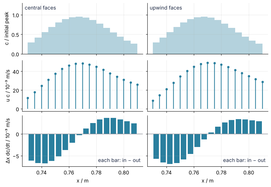
The face fluxes differ between the columns. Each upwind face takes the cell behind it, so its flux is smaller than the central one on the left flank of the pulse and larger on the right. The rule does not differ. In both columns each bar in the bottom row is the stem on its left minus the stem on its right, and whatever one cell loses, its neighbor gains.

Now the three runs side by side, all the way through the pipe:

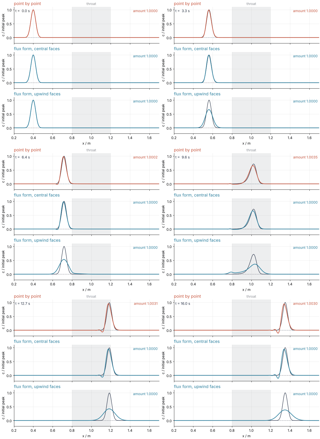
How I built this: Matplotlib animation with FuncAnimation: a probe sweep as a small GIF; the source is animations/pulses/scene.py.

The two flux runs hold their amount at 1.0000 from start to finish. Their shapes are not the same, though, and that is the subject of the next section.

The face value: central average or upwind

With central faces, the cell downstream has a say in what leaves the cell upstream. For a pulse only five cells wide that is too much say: the pulse leaves a train of ripples behind it, and the ripples dip below zero. Negative dye is not in the physics. The Formalization says where the ripples come from.

With upwind faces, a cell only ever gives away a share of what it already holds, so it can never go negative, provided the time step is short enough (the Courant number in the Formalization says how short). The price is that the face value lags half a cell behind the true one, and the pulse smears out as it travels.

Show code

Copy

c_upwind, amount_upwind, _ = run(lambda c: flux_rate(c, "upwind"))
c_exact = exact(x, t_end)

print(f"central faces    minimum {c_central.min():+.3f}   peak {c_central.max():.3f}")
print(f"upwind faces     minimum {c_upwind.min():+.3f}   peak {c_upwind.max():.3f}")
print(f"exact            peak {c_exact.max():.3f} at the cell centers")
for name, a in [("point by point", amount_point), ("central faces", amount_central), ("upwind faces", amount_upwind)]:
    print(f"{name:15s}  amount change {a[-1] / a[0] - 1:+.1e}")
print(f"dye in the three cells at either end: {max(abs(c_upwind[:3]).max(), abs(c_upwind[-3:]).max()):.0e}")

fig = plt.figure(figsize=(8, 5), layout="constrained")
gs = fig.add_gridspec(3, 2, width_ratios=[1.1, 1])
runs = [("point by point", c_point, ACCENT), ("central faces", c_central, SECOND), ("upwind faces", c_upwind, SECOND)]
ax_left = None
for row, (name, c_run, color) in enumerate(runs):
    ax = fig.add_subplot(gs[row, 0], sharex=ax_left, sharey=ax_left)
    ax_left = ax_left or ax
    ax.axhline(0, color=MUTED, lw=1, ls="--")
    ax.plot(x, c_exact, color=INK, lw=1.2)
    ax.plot(x, c_run, color=color)
    ax.text(0.02, 0.92, name, transform=ax.transAxes, va="top", color=color)
    ax.set(ylabel="c / initial peak", xlim=(1.15, 1.55), ylim=(-0.2, 1.1))
    if row < 2:
        ax.tick_params(labelbottom=False)
ax.text(1.372, 0.88, "exact", color=INK, va="center")
ax.set_xlabel("x / m")
ax_amt = fig.add_subplot(gs[:, 1])
ax_amt.axvspan(*t_throat, color=MUTED, alpha=0.15, lw=0)
ax_amt.text(np.mean(t_throat), 0.15, "pulse\nin throat", ha="center", va="center", color=MUTED)
ax_amt.plot(t_steps, drift_point, color=ACCENT)
ax_amt.plot(t_steps, 100 * (amount_central / amount_central[0] - 1), color=SECOND)
ax_amt.plot(t_steps, 100 * (amount_upwind / amount_upwind[0] - 1), color=SECOND, ls=":")
ax_amt.annotate(f"point by point\n{drift_point[-1]:+.2f} %", (t_end, drift_point[-1]), xytext=(0, -8),
                textcoords="offset points", color=ACCENT, ha="right", va="top")
ax_amt.text(t_end, 0.02, "both flux runs", color=SECOND, ha="right", va="bottom")
ax_amt.set(xlabel="t / s", ylabel="amount change / %", xlim=(0, t_end))
plt.show()

central faces    minimum -0.109   peak 0.945
upwind faces     minimum +0.000   peak 0.381
exact            peak 0.995 at the cell centers
point by point   amount change +3.0e-03
central faces    amount change -4.5e-14
upwind faces     amount change -4.3e-14
dye in the three cells at either end: 3e-18

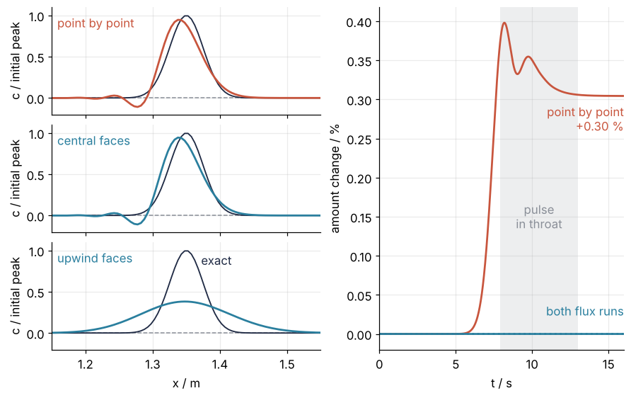
Central dips to −0.109 and peaks at 0.945. Upwind stays positive everywhere, but its peak is 0.381 against 0.995 for the exact pulse at the cell centers. The point-by-point run has the same ripples as central, because it uses the same central difference. Only its books are off.

Formalization

Write \(\bar c_i\) for the average \((1/\Delta x)\int c\,dx\) over cell \(i\), the array above. Integrating the law over the cell is exact:

with \(F = uc\) at the faces on either side. Nothing is approximated yet: only the face value and the time step will be.

Conservation is a telescoping sum. Summed over all cells, every inner face appears twice, once with each sign, and only \(F_\text{in} - F_\text{out}\) at the pipe ends survives. Both are zero here, so the amount changes by rounding alone. Multiply the point-by-point update by \(\Delta x\) and sum it the same way:

The first sum does not telescope, because \(u\) changes from cell to cell, and the second is not a difference at all. Rename the index in each half of the first, \(\sum_i u_i c_{i+1} = \sum_i u_{i-1} c_i\) and \(\sum_i u_i c_{i-1} = \sum_i u_{i+1} c_i\), since the end cells hold no dye. That moves the difference from \(c\) onto \(u\):

The bracket is the central-difference slope of \(u\) minus its true slope, weighted by the dye. To leading order it is \((\Delta x^2/6)\,u'''\), which is large at the entry and the exit of the throat. That says where the leak shows, not why there is one. Take \(du/dx\) by the same central difference as \(\partial c/\partial x\), less accurate than the formula, and the bracket vanishes: the update becomes a difference of the face fluxes \((u_i c_{i+1} + u_{i+1} c_i)/2\) and conserves exactly. The form decides, not the accuracy: an update conserves when it is a difference of face fluxes, and the flux form passes that test on every grid and for every face value.

Numerical diffusion. For \(u > 0\) the upwind face value is the cell whose center lies half a cell behind the face. By Taylor expansion \(\bar c_i = c(x_{i+1/2}) - (\Delta x/2)\,\partial c/\partial x + \dots\), so the upwind flux is

and the second term is Fick's law with a diffusion coefficient \(D = u\Delta x/2\). Upwind solves the law plus a diffusion nobody put in. In the wide pipe \(D\) = 1.25 × 10⁻⁴ m²/s, some 300,000 times the value for fluorescein in water.

The number checks out. Diffusion adds \(2Dt\) to the variance of a Gaussian, the random-walk law. In that time the pulse moves \(s = ut\), so \(2Dt = u\Delta x \cdot s/u = \Delta x\, s\): \(u\) cancels, and the variance grows by \(\Delta x\) per meter traveled, at any speed.

The only throat factor is the stretch. Smear added in the throat lands on a pulse stretched by \(u/u_0\), and when the pulse contracts again that variance shrinks by \((u_0/u)^2\), so a meter of throat counts only \((u_0/u)^2\) as much. Along the path, \(\Delta x \int (u_0/u)^2\,dx\) = 5 mm × 0.73 m (of 0.95 m traveled), which takes \(\sigma\) from 2.5 to 6.56 cm and the peak to 1.000 × 2.5/6.56 = 0.381, against 0.381 computed. The 1.000 is the exact pulse's true peak. Its narrow top reads only 0.995 at the cell centers, a loss the smeared pulse is too wide to suffer:

D_num = u0 * dx / 2
x_center = np.interp(np.interp(x0, x_fine, tau) + t_end, tau, x_fine)      # where the exact pulse is at t_end
path = (x_fine > x0) & (x_fine < x_center)
path_eff = np.trapezoid((u0 / speed(x_fine[path]))**2, x_fine[path])
sigma_end = np.sqrt(sigma0**2 + dx * path_eff)
peak_exact = exact(x_fine, t_end).max()                                    # the true peak, not the one at the cell centers
print(f"numerical diffusion  D = u0 dx / 2 = {D_num:.2e} m^2/s")
print(f"path                 {x_center - x0:.2f} m traveled, {path_eff:.2f} m effective")
print(f"pulse width          sigma {100 * sigma0:.2f} cm -> {100 * sigma_end:.2f} cm")
print(f"upwind peak          predicted {peak_exact * sigma0 / sigma_end:.3f}, computed {c_upwind.max():.3f}")

numerical diffusion  D = u0 dx / 2 = 1.25e-04 m^2/s
path                 0.95 m traveled, 0.73 m effective
pulse width          sigma 2.50 cm -> 6.56 cm
upwind peak          predicted 0.381, computed 0.381

Numerical diffusion grows with the cell size, and it looks exactly like real mixing. Never fit a dispersion coefficient to an upwind result before you have halved the cells and seen whether it changes.

Central's leading error in the equation is a third derivative, and it does not smear. Write the pulse as a sum of sine waves, its Fourier series. On a wave \(e^{ikx}\) the derivative is a factor \(ik\) and the central difference \(i\sin(k\Delta x)/\Delta x \approx i(k - k^3\Delta x^2/6)\), whose \(k^3\) term is that third derivative. So in constant flow the wave keeps its amplitude but travels at \(u\sin(k\Delta x)/(k\Delta x)\), the slower the shorter it is: a wave four cells long moves at 0.64 \(u\) and falls behind into the trailing ripples.

The Courant number. A forward Euler step, \(\bar c_i \leftarrow \bar c_i + (\Delta t/\Delta x)(F_{i-1/2} - F_{i+1/2})\), turns the cell equation into a time step. With upwind faces in constant flow it reads

where the Courant number \(C\) is the fraction of a cell the water crosses in one step. With \(C \le 1\) the new value is a weighted average of old ones: no negative dye and no new maxima. Beyond 1, a cell gives away more than it holds. Here \(\Delta t\) = 13.6 ms gives \(C\) = 0.5 where the water is fastest. The same number sets the time step for waves on a string with leapfrog.

With central faces a single Euler step would multiply each wave by \(\sqrt{1 + C^2 \sin^2 k\Delta x}\), 1.12 for the four-cell wave at \(C\) = 0.5. The runs use the three-stage Runge-Kutta method of Shu and Osher instead, an average of Euler stages that keeps the books and upwind's positivity and takes that factor to 0.998. Central stays bounded, and its ripples are the dispersion above, not growth.

See it in code

Here is the whole method in its compact form. np.diff of the face fluxes is the telescoping sum; divided by \(\Delta x\) it is each cell's rate of change, which the three Runge-Kutta stages advance, not a single Euler step. It runs on the grid above and on one twice as fine:

def finite_volume(c, u_face, dx, dt, n_steps, face):
    """Advance the cell averages c; u_face holds the speed at the len(c) + 1 faces."""
    def fv_rate(c):
        cp = np.pad(c, 1)
        c_left, c_right = cp[:-1], cp[1:]
        c_face = 0.5 * (c_left + c_right) if face == "central" else np.where(u_face > 0, c_left, c_right)
        return -np.diff(u_face * c_face) / dx
    for _ in range(n_steps):
        c = rk3_step(c, fv_rate, dt)
    return c

print(" dx/mm   point drift   flux drift   central min   upwind peak   predicted   exact")
for refine in (1, 2):
    h, k, steps = dx / refine, dt / refine, n_steps * refine           # same Courant number on both grids
    xc, xf = (np.arange(N * refine) + 0.5) * h, np.arange(N * refine + 1) * h
    uc, duc = speed(xc), dudx(xc)
    point = lambda c: -uc * (np.pad(c, 1)[2:] - np.pad(c, 1)[:-2]) / (2 * h) - c * duc
    c = pulse(xc)
    for _ in range(steps):
        c = rk3_step(c, point, k)
    point_drift = c.sum() / pulse(xc).sum() - 1
    cen = finite_volume(pulse(xc), speed(xf), h, k, steps, "central")
    upw = finite_volume(pulse(xc), speed(xf), h, k, steps, "upwind")
    flux_drift = max(abs(cen.sum() / pulse(xc).sum() - 1), abs(upw.sum() / pulse(xc).sum() - 1))
    ex = exact(xc, t_end).max()
    predicted = peak_exact * sigma0 / np.sqrt(sigma0**2 + h * path_eff)
    print(f"{1e3 * h:6.2f}   {100 * point_drift:+9.3f} %   {flux_drift:9.0e}   {cen.min():+11.4f}"
          f"   {upw.max():11.3f}   {predicted:9.3f}   {ex:5.3f}")

 dx/mm   point drift   flux drift   central min   upwind peak   predicted   exact
  5.00      +0.304 %       4e-14       -0.1085         0.381       0.381   0.995
  2.50      +0.075 %       9e-14       -0.0010         0.504       0.504   0.999

The point-by-point drift falls fourfold, from 0.30 % to 0.075 %, which is second order at work, but a finer grid shrinks the leak without closing it. The flux form stays at rounding on both grids. Central's ripples fade from −0.109 to −0.001, a tenth of a percent of the peak, once the pulse is ten cells wide, so central faces are the better choice when the narrowest feature spans about ten cells or more.

Halving the cells lifts upwind's peak only from 0.38 to 0.50, as \(u\Delta x/2\) predicts: the added variance halves when the cells do and no faster, which is what first order means. So upwind is the choice when the quantity must stay positive (a concentration that feeds a chemistry model) or the fronts are only a few cells wide. Because the code takes the cell the water comes from face by face, by the sign of \(u\), it holds where the flow reverses too. When dye flows in, pad the inlet side with the inflow concentration instead of zero: with upwind faces the first face then carries exactly what enters, and the value beyond the outlet is never read.

Where it shows up

• Groundwater and contaminant transport. MODFLOW 6, the U.S. Geological Survey's groundwater code, keeps a water budget for every cell, and its transport model moves solutes between cells with an upstream, central, or TVD face value, the same choice as above. The flux through each face comes from Darcy's law, as in findiff.PDE with mixed boundary conditions: seepage under a dam.
• Atmosphere and ocean. The FV3 dynamical core of NOAA's Global Forecast System and MITgcm, widely used for the ocean, are finite volume codes. A climate run lasts a hundred years, and a gain of 0.30 % each time air passes a feature would compound over thousands of passages into mass the model invented.
• Combustion and engineering flow. OpenFOAM and Ansys Fluent discretize every transported quantity by finite volumes. A negative mass fraction from central ripples breaks the chemistry, which is why such codes offer bounded face values that blend central and upwind.
• Traffic flow. Daganzo's cell transmission model counts cars per road cell and moves them across cell boundaries. The flux is limited by what the cell upstream can send and what the cell downstream can take.
• Floods and tsunamis. GeoClaw, part of Clawpack, and the 2D solver of HEC-RAS are finite volume codes: the water in each cell changes by what flows through its faces. A water depth that goes negative is as useless as negative dye, so the face value is picked with care there too.

In every case whatever leaves one cell enters its neighbor, and the face value decides between ripples and smear.

Further reading

• numpy.diff, the one function the method needs.
• FiPy, when you want the method without writing it.
• LeVeque, Finite Volume Methods for Hyperbolic Problems (Cambridge, 2002), for face values beyond central and upwind.
• Patankar, Numerical Heat Transfer and Fluid Flow (1980), the control-volume classic.
• Other PDE tutorials on this site: The wave equation with leapfrog finite differences: a pulse on a string; findiff.PDE with mixed boundary conditions: seepage under a dam; py-pde from the ground up: the heat equation on a square plate; Devito from the ground up: a seismic shot over a buried reflector.
• Surface temperature of an airless planet: day, night, and below the ground, whose right-hand side is flux in minus flux out, a finite volume grid in disguise.
• Stiffness: why an explicit solver crawls on a reaction that has long settled, for more on explicit time steps, and Matplotlib animation with FuncAnimation: a probe sweep as a small GIF.
• Planned: the finite differences Concept, FiPy from the ground up, and Finite volumes in Julia.
• Download the notebook. It was executed with the library versions in the header.