Kriging with PyKrige: a groundwater map from forty wells and how sure it is

The problem: a groundwater map from forty wells, and where to trust it

Forty observation wells are scattered over a 10 km × 10 km catchment, and each gives one groundwater level, between 114.3 and 122.3 m above sea level. You need the level everywhere, as a map. Before you site a new well you also need to know how far to trust that map at a spot where no well stands. Kriging answers both questions. It estimates the level at any point as a weighted sum of the well levels, with weights taken from the variogram, a curve that says how much the levels at two points differ, on average, as a function of the distance between them. With every estimate it returns a variance, which is zero at a well and largest far from all of them.

The wells here are drawn from a made-up field whose true level is known at each of 2,601 map nodes, so the map can be checked against the truth instead of taken on trust. The kriging is done by PyKrige, the variogram is fitted with curve_fit, and SciPy's griddata provides the plain alternative to beat, linear interpolation between the wells.

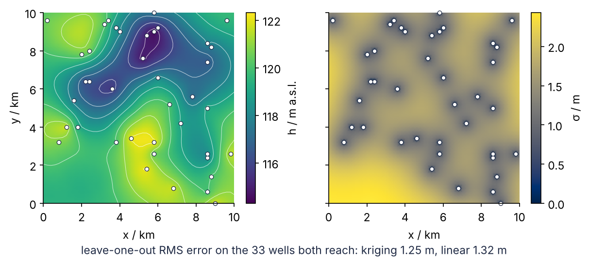
This is where we end up: the kriged level on the left, its standard deviation on the right. Left out one at a time and predicted from the other 39, the wells come back with an RMS error of 1.25 m from kriging and 1.32 m from linear interpolation. That gain is small, and it changes with where the wells happen to fall. The reasons to krige are a map of the whole catchment and an uncertainty that turns out to be the right size.

Setup

The first half of the block loads the tools. The second half builds the test catchment, and its machinery uses the very variogram this tutorial is about, so this is the one place where the code runs ahead of the text: run it now, and the steps explain what they need from it. The function spherical and its three parameters return in Step 3, and the true field truth stays aside until Step 6. In the field you would have only the three arrays xw, yw, hw.

# ---- tools
import numpy as np
import matplotlib.pyplot as plt
from scipy.spatial.distance import cdist
from scipy.optimize import curve_fit
from scipy.interpolate import griddata
from pykrige.ok import OrdinaryKriging

plt.rcParams.update({
    "figure.figsize": (7, 3.6), "figure.dpi": 110,
    "axes.spines.top": False, "axes.spines.right": False,
    "axes.grid": True, "grid.alpha": 0.25,
    "font.size": 11, "lines.linewidth": 1.8,
})
INK, ACCENT, SECOND, MUTED = "#1f2a44", "#c8553d", "#2a7f9e", "#8a8f98"

# ---- a made-up catchment whose true levels we know
MEAN, SILL, RANGE = 120.0, 4.0, 4.0      # m a.s.l., m², km
rng = np.random.default_rng(2026)
gx = gy = np.linspace(0, 10, 51)         # map nodes every 200 m, in km
X, Y = np.meshgrid(gx, gy)
nodes = np.column_stack([X.ravel(), Y.ravel()])

def spherical(h, psill, range_km, nugget):                     # Step 3
    h = np.asarray(h, dtype=float)
    rise = np.where(h < range_km, 1.5 * h / range_km - 0.5 * (h / range_km) ** 3, 1.0)
    return nugget + psill * rise

cov = SILL - spherical(cdist(nodes, nodes), SILL, RANGE, 0.0)   # covariance from the variogram
chol = np.linalg.cholesky(cov + 1e-8 * np.eye(len(nodes)))      # tiny jitter for round-off
truth = MEAN + chol @ rng.standard_normal(len(nodes))           # Step 6
idx = rng.choice(len(nodes), 40, replace=False)
xw, yw, hw = nodes[idx, 0], nodes[idx, 1], truth[idx]           # the wells: x, y in km, level in m

print(f"{len(nodes)} map nodes, {len(hw)} wells, levels {hw.min():.1f} to {hw.max():.1f} m")

2601 map nodes, 40 wells, levels 114.3 to 122.3 m

Step 1: Look at the wells and list their pairs

Plot the wells colored by level, with viridis, a colormap whose brightness rises evenly with the value:

Copy

fig, ax = plt.subplots(figsize=(4.5, 4))
sc = ax.scatter(xw, yw, c=hw, cmap="viridis", s=45, edgecolor=INK, lw=0.6, zorder=3)
fig.colorbar(sc, ax=ax, label="h / m a.s.l.")
ax.set(xlabel="x / km", ylabel="y / km", xlim=(-0.3, 10.3), ylim=(-0.3, 10.3), aspect="equal")
plt.show()

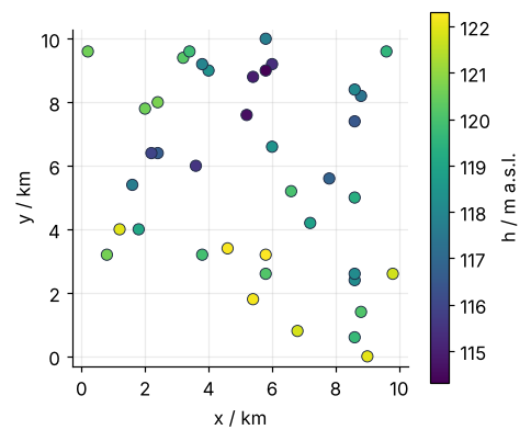
Wells close together tend to share a color: the four lowest, all below 115.5 m, lie within 2 km of each other, and the six highest all lie in the lower half. The variogram puts a number on that, and it is built from pairs of wells. np.triu_indices returns two arrays, i and j, holding the two well numbers of every pair:

i, j = np.triu_indices(len(hw), k=1)
d = np.hypot(xw[i] - xw[j], yw[i] - yw[j])        # distance of each pair, km
print(f"{d.size} pairs, shortest {d.min():.1f} km, longest {d.max():.1f} km")

780 pairs, shortest 0.2 km, longest 13.0 km

Forty wells make 780 pairs. The variogram is estimated from the pairs, not from the wells, which is why forty wells are enough at all.

Step 2: Bin the pairs into an experimental variogram

Half the squared difference of the two levels is the semivariance of a pair. It is computed with the same index arrays, so entry k of sv and entry k of d belong to the same pair of wells. Averaged over the pairs at similar distance, it gives the experimental semivariogram

where the sum runs over the \(N(h)\) pairs whose distance falls in the bin around \(h\), and \(z_i\) is the level at well \(i\). Bins of 0.5 km up to 6 km:

Copy

sv = 0.5 * (hw[i] - hw[j]) ** 2
edges = np.arange(0, 6.01, 0.5)
b = np.digitize(d, edges) - 1
keep = b < len(edges) - 1                          # pairs farther than 6 km are dropped
N = np.bincount(b[keep], minlength=len(edges) - 1)
h = np.bincount(b[keep], weights=d[keep], minlength=len(edges) - 1) / N      # mean distance per bin
gamma = np.bincount(b[keep], weights=sv[keep], minlength=len(edges) - 1) / N

print("  h / km   γ / m²   pairs")
for hk, gk, nk in zip(h, gamma, N):
    print(f"  {hk:5.2f}   {gk:6.2f}   {nk:5d}")

fig, ax = plt.subplots()
ax.plot(h, gamma, "o", color=INK, ms=6)
for hk, gk, nk in zip(h, gamma, N):
    ax.annotate(str(nk), (hk, gk), xytext=(5, 4), textcoords="offset points", color=MUTED)
ax.set(xlabel="distance h / km", ylabel="semivariance γ / m²", xlim=(0, 6.2), ylim=(0, None))
plt.show()

  h / km   γ / m²   pairs
   0.30     0.18       8
   0.78     1.90      15
   1.28     3.33      25
   1.72     2.71      24
   2.25     4.00      45
   2.73     6.57      40
   3.27     3.80      67
   3.76     7.07      48
   4.22     4.73      47
   4.77     4.71      52
   5.21     4.71      49
   5.75     6.87      59

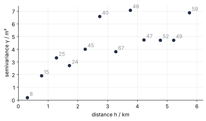
The semivariance rises from 0.18 m² in the first bin to a plateau near 5 m² beyond about 4 km. The first bin holds eight pairs, the busiest 67. The cutoff at 6 km is about half the largest distance: beyond it the pairs thin out, and the ones left are all wells near opposite edges.

Step 3: Fit a variogram model: nugget, sill, and range

Kriging needs the variogram at every distance, so a smooth model replaces the dots. Three numbers describe it. The nugget is the jump at zero distance, from measurement error and variation on scales shorter than the well spacing. The sill is the plateau, the variance of the level. The range is the distance beyond which two levels are unrelated. The partial sill is the sill minus the nugget, the height of the rise above the jump; PyKrige and the code call it psill. The spherical model rises linearly near zero and reaches the sill exactly at the range, the exponential starts twice as steep and approaches the sill only gradually, and the Gaussian starts flat.

Fit all three with curve_fit, as in curve_fit from the ground up. A bin mean over N pairs scatters about as \(1/\sqrt N\), so sigma=1/np.sqrt(N) makes the bins with many pairs count more:

Copy

def exponential(h, psill, range_km, nugget):     # PyKrige's form: 95 % of the rise at the range
    return nugget + psill * (1 - np.exp(-3 * h / range_km))

def gaussian(h, psill, range_km, nugget):        # PyKrige's form: 95 % of the rise at the range, too
    return nugget + psill * (1 - np.exp(-(h / (4 / 7 * range_km)) ** 2))

models = {"spherical": spherical, "exponential": exponential, "gaussian": gaussian}
fits = {}
print("model         psill   nugget   sill / m²   range / km")
for name, model in models.items():
    p, _ = curve_fit(model, h, gamma, p0=[gamma.max(), 3, 0.1], sigma=1 / np.sqrt(N),
                     bounds=([0, 0.1, 0], [20, 20, 5]))
    fits[name] = {"psill": p[0], "range": p[1], "nugget": p[2]}
    print(f"{name:12s} {p[0]:6.2f}  {p[2]:6.2f}   {p[0] + p[2]:8.2f}   {p[1]:9.2f}")
print(f"{'truth':12s} {SILL:6.2f}  {0:6.2f}   {SILL:8.2f}   {RANGE:9.2f}")

sph = fits["spherical"]
hh = np.linspace(0, 6.2, 300)
fig, ax = plt.subplots()
ax.plot(h, gamma, "o", color=INK, ms=6, label="binned pairs")
ax.plot(hh, spherical(hh, sph["psill"], sph["range"], sph["nugget"]), color=ACCENT, label="spherical fit")
e = fits["exponential"]
ax.plot(hh, exponential(hh, e["psill"], e["range"], e["nugget"]), color=SECOND, label="exponential fit")
ax.plot(hh, spherical(hh, SILL, RANGE, 0.0), color=MUTED, ls="--", lw=1.2, label="true model")
sill = sph["psill"] + sph["nugget"]
ax.axhline(sill, color=MUTED, lw=0.8, ls=":")
ax.axvline(sph["range"], color=MUTED, lw=0.8, ls=":")
ax.text(0.1, sill + 0.15, "sill = nugget + partial sill", color=MUTED)
ax.text(sph["range"] + 0.08, 7.5, "range", color=MUTED)
ax.annotate("nugget", (0, sph["nugget"]), xytext=(0.75, 0.55), color=MUTED,
            arrowprops=dict(arrowstyle="-", color=MUTED, lw=0.8))
ax.set(xlabel="distance h / km", ylabel="semivariance γ / m²", xlim=(0, 6.2), ylim=(0, 8))
ax.legend(frameon=False, loc="lower right")
plt.show()

model         psill   nugget   sill / m²   range / km
spherical      5.22    0.26       5.48        3.94
exponential    6.04    0.00       6.04        5.62
gaussian       4.53    0.95       5.48        3.32
truth          4.00    0.00       4.00        4.00

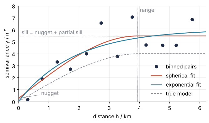
The spherical fit puts the range at 3.94 km, against the true 4 km. Its sill, 5.48 m², lies above the true 4 m². The rules in Setup could build endless catchments, and 4 m² is the variance averaged over all of them; truth is one random draw, and it happens to vary more than the average. PyKrige fits a model on its own when you leave out the parameters:

auto = OrdinaryKriging(xw, yw, hw, variogram_model="spherical")
print(np.round(auto.variogram_model_parameters, 2))

[5.07 3.78 0.  ]

The list is partial sill, range, and nugget: 5.07 m², 3.78 km, and zero, close to the hand fit. I keep the spherical model; Step 5 checks it against the other two.

Step 4: Krige onto the grid with OrdinaryKriging

Ordinary kriging writes the estimate at a point \(x_0\) as a weighted sum of the \(n\) well levels,

The weights sum to one because the mean of the field is unknown, and any constant mean must pass through unchanged. Of all such weights, kriging picks the ones that make the expected squared error, \((\hat z(x_0) - z(x_0))^2\) averaged over every field with this variogram, as small as possible. That smallest value is the kriging variance, and its square root is the typical error the model expects at \(x_0\). The weights solve a linear system built from the variogram between all pairs of wells and between each well and \(x_0\), with one extra unknown that enforces the sum of one. Pass the fitted model as a dict: the list form of variogram_parameters wants the full sill, not the partial sill that variogram_model_parameters returns, so a list passed back silently changes the model.

ok = OrdinaryKriging(xw, yw, hw, variogram_model="spherical", variogram_parameters=fits["spherical"])

px, py = np.array([xw[0], 0.0, 10.0]), np.array([yw[0], 0.0, 10.0])
z_pts, ss_pts = ok.execute("points", px, py)
sd_pts = np.sqrt(np.clip(ss_pts, 0, None))        # the variance is a hair below 0 at some wells
for label, z, s in zip(["well 0", "(0, 0)", "(10, 10)"], z_pts, sd_pts):
    print(f"{label:9s} {z:7.2f} ± {s:.2f} m")
print(f"well 0 measured {hw[0]:.2f} m;  mean of the wells {hw.mean():.2f} m;  √sill {np.sqrt(sill):.2f} m")

z_grid, ss_grid = ok.execute("grid", gx, gy)
sd_grid = np.sqrt(np.clip(ss_grid, 0, None))
print(f"grid {z_grid.shape}, smallest variance {ss_grid.min():.0e} m², largest σ {sd_grid.max():.2f} m")

well 0     118.16 ± 0.00 m
(0, 0)     119.44 ± 2.43 m
(10, 10)   119.66 ± 1.56 m
well 0 measured 118.16 m;  mean of the wells 118.90 m;  √sill 2.34 m
grid (51, 51), smallest variance -7e-14 m², largest σ 2.43 m

Both calls return masked arrays; with no mask given nothing is hidden, and plain arithmetic works. At a well the map returns the measured level with zero standard deviation, because exact_values=True is the default. At (0, 0), far from the wells, the estimate falls back toward their mean, and the standard deviation rises to 2.43 m, a little past the square root of the sill, 2.34 m, because ordinary kriging also carries the uncertainty of the unknown mean.

Step 5: Cross-validate the map and the model by leaving one well out

Leave-one-out cross-validation tests a map on the wells themselves: take one well out, krige its spot from the other 39, compare, and repeat for all 40. The variogram stays as fitted in Step 3, since one well removes only 39 of its 780 pairs. The loop runs over all three models.

Linear interpolation gets the same test. It fills triangles between wells with flat planes, so it answers only inside the convex hull of the wells, the outline of a rubber band stretched around them. A well on the edge of the network, left out, lies outside the hull of the other 39.

Dividing each kriging error by its standard deviation gives a standardized error. If the standard deviation is the right size, these have a mean square near 1 and about 95 % of them, 38 of 40, lie within ±2. Below 1 means the errors are smaller than predicted, a cautious map; above 1, an overconfident one.

err, sd = {}, {}
for name in models:
    err[name], sd[name] = np.empty(40), np.empty(40)
    for k in range(40):
        rest = np.arange(40) != k
        ok_k = OrdinaryKriging(xw[rest], yw[rest], hw[rest], variogram_model=name,
                               variogram_parameters=fits[name])
        z_k, ss_k = ok_k.execute("points", xw[k:k + 1], yw[k:k + 1])
        err[name][k], sd[name][k] = z_k[0] - hw[k], np.sqrt(ss_k[0])

err_lin = np.empty(40)
for k in range(40):
    rest = np.arange(40) != k
    err_lin[k] = griddata((xw[rest], yw[rest]), hw[rest], (xw[k], yw[k]), method="linear") - hw[k]
reach = ~np.isnan(err_lin)                          # NaN: outside the hull of the other 39

rms = lambda e: np.sqrt(np.mean(e ** 2))
print(f"method        RMS, 40 wells   RMS, {reach.sum()} wells   mean z²   |z| ≤ 2")
for name in models:
    z = err[name] / sd[name]                        # standardized errors
    print(f"{name:12s} {rms(err[name]):9.2f} m {rms(err[name][reach]):11.2f} m"
          f" {np.mean(z ** 2):9.2f} {np.sum(np.abs(z) <= 2):6d} of 40")
print(f"{'linear':12s} {'-':>11s} {rms(err_lin[reach]):11.2f} m      {(~reach).sum()} wells out of reach")

for name in ["exponential", "gaussian"]:            # a gap between models, and its standard error
    diff = err[name] ** 2 - err["spherical"] ** 2
    print(f"{name} minus spherical, mean squared error: "
          f"{diff.mean():+.2f} ± {diff.std(ddof=1) / np.sqrt(40):.2f} m²")

method        RMS, 40 wells   RMS, 33 wells   mean z²   |z| ≤ 2
spherical         1.33 m        1.25 m      0.73     40 of 40
exponential       1.35 m        1.31 m      0.66     40 of 40
gaussian          1.31 m        1.21 m      0.73     40 of 40
linear                 -        1.32 m      7 wells out of reach
exponential minus spherical, mean squared error: +0.05 ± 0.11 m²
gaussian minus spherical, mean squared error: -0.05 ± 0.07 m²

Linear interpolation cannot reach seven wells. Mean squares of 0.66 to 0.73, with all 40 errors inside ±2, put the standard deviation on the cautious side. The models differ by 0.04 m in RMS. The last two lines test that gap. At each well they subtract the squared error of spherical from that of the other model, which cancels the wells that are hard for every model, and average: exponential is worse by 0.05 m², Gaussian better by 0.05 m². The ± is the standard error of that average, how far it would move with another forty wells, and at 0.11 and 0.07 m² it exceeds both gaps. Forty wells cannot tell these models apart. Keep spherical, the usual model when the variogram reaches a clear plateau, and switch only for a gap of twice its standard error or more.

Step 6: Check against the truth and draw the map with its uncertainty

Now the truth from Setup, on the map nodes inside the convex hull of all 40 wells, exactly the nodes where griddata returns a number:

true_map = truth.reshape(X.shape)
z_lin = griddata((xw, yw), hw, (X, Y), method="linear")
inside = ~np.isnan(z_lin)
rms_map = lambda m: np.sqrt(np.mean((m - true_map)[inside] ** 2))

print(f"RMS against the truth inside the hull: kriging {rms_map(z_grid):.2f} m, linear {rms_map(z_lin):.2f} m")
print(f"linear leaves {100 * (1 - inside.mean()):.1f} % of the catchment blank")
covered = np.abs(true_map - z_grid) <= 2 * sd_grid
print(f"true level within ±2 kriging σ: {100 * covered.mean():.1f} % of the nodes")
q10, q50, q90 = np.percentile(np.asarray(sd_grid)[inside], [10, 50, 90])
print(f"kriging σ inside the hull: median {q50:.2f} m, 10th to 90th percentile {q10:.2f} to {q90:.2f} m")
others = {name: OrdinaryKriging(xw, yw, hw, variogram_model=name, variogram_parameters=fits[name])
          .execute("grid", gx, gy)[0] for name in ["exponential", "gaussian"]}
print("other models: " + ", ".join(f"{n} {rms_map(m):.2f} m" for n, m in others.items()))

RMS against the truth inside the hull: kriging 1.04 m, linear 1.14 m
linear leaves 27.1 % of the catchment blank
true level within ±2 kriging σ: 97.5 % of the nodes
kriging σ inside the hull: median 1.45 m, 10th to 90th percentile 1.09 to 1.73 m
other models: exponential 1.05 m, gaussian 1.06 m

Then the map, the level in viridis and the standard deviation in cividis, so the panels cannot be read as one quantity:

Copy

fig, (ax1, ax2) = plt.subplots(1, 2, figsize=(8, 3.3), sharex=True, sharey=True, layout="constrained")
fig.get_layout_engine().set(wspace=0.08)           # room between the left colorbar and the right panel
m1 = ax1.pcolormesh(gx, gy, z_grid, cmap="viridis", shading="gouraud")
ax1.contour(gx, gy, z_grid, levels=np.arange(114, 124), colors="white", linewidths=0.5, alpha=0.7)
fig.colorbar(m1, ax=ax1, label="h / m a.s.l.", pad=0.03)
m2 = ax2.pcolormesh(gx, gy, sd_grid, cmap="cividis", shading="gouraud")
fig.colorbar(m2, ax=ax2, label="σ / m", pad=0.03)
for ax in (ax1, ax2):
    ax.plot(xw, yw, "o", ms=4, mfc="white", mec=INK, mew=0.6, clip_on=False)
    ax.set(xlabel="x / km", aspect="equal")
    ax.grid(False)
ax1.set_ylabel("y / km")
fig.text(0.5, -0.04, f"leave-one-out RMS error on the {reach.sum()} wells both reach: "
         f"kriging {rms(err['spherical'][reach]):.2f} m, linear {rms(err_lin[reach]):.2f} m",
         ha="center", color=INK)
plt.show()

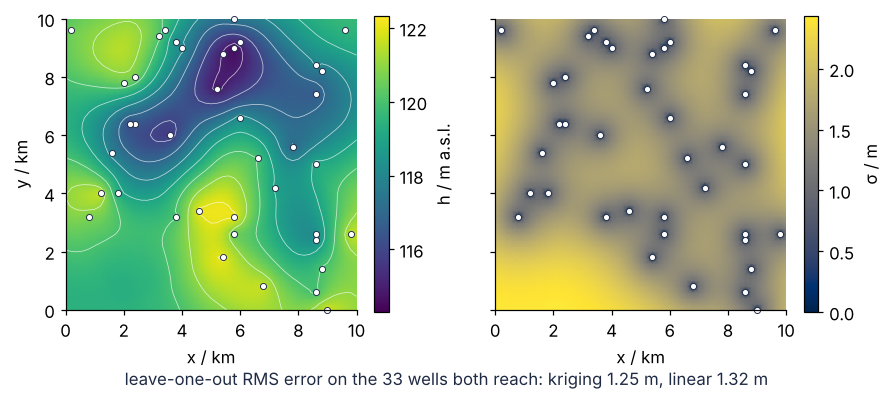
Kriging beats linear interpolation slightly on both tests: 1.25 against 1.32 m on the left-out wells, 1.04 against 1.14 m against the truth. Its standard deviation is the right size, a little cautious: the mean square of 0.73 lies below 1, the coverage of 97.5 % above 95 %. The exponential and Gaussian maps land at 1.05 and 1.06 m, so the choice of model cost nothing. Over this seed and four others, a run not shown here, the gain against the truth ranged from nothing to 15 %. The gain is not the reason to krige. Linear interpolation leaves 27.1 % of the catchment blank and gives no uncertainty at all. The right panel answers the siting question: a dimple at every well, a median of 1.45 m inside the hull, and 2.43 m in the lower left corner.

Pitfalls

A trend the variogram cannot see past. The experimental variogram keeps rising and never levels off. The cause is a regional gradient, groundwater sloping toward a river, which ordinary kriging, with its constant unknown mean, assumes away. Add a slope of 0.5 m per km to the levels and bin in 2 km steps:

b2 = (d // 2).astype(int)                          # 2 km bins, 0 to 10 km
for label, levels in [("as measured", hw), ("with trend", hw + 0.5 * xw)]:
    sv2 = 0.5 * (levels[i] - levels[j]) ** 2
    g2 = [sv2[b2 == k].mean() for k in range(5)]
    print(f"{label:12s}", "  ".join(f"{g:5.1f}" for g in g2), "m²")

as measured    2.5    5.2    5.3    6.1    5.8 m²
with trend     2.3    5.1    6.5    8.0   11.9 m²

With the trend the semivariance climbs past twice the plateau. Use UniversalKriging from pykrige.uk with drift_terms=["regional_linear"] (drift is PyKrige's word for the trend), or remove the trend yourself and krige the residuals.

Too few pairs in the first bins. The nugget and the shape near zero jump when you change the bin width. The behavior at short distance matters most for the weights, and in Step 2 it rests on the eight pairs of the first bin. Look at the pair counts before you fit, widen the first bins, and weight by N. When you design the network yourself, place a few wells in close pairs.

Reading the kriging variance as a measured error. The map looks confident where the levels are erratic and doubtful where they are smooth. The kriging variance depends only on the well positions and the variogram model, never on the levels themselves. Shuffle the levels among the wells and krige again:

ok_shuffled = OrdinaryKriging(xw, yw, rng.permutation(hw), variogram_model="spherical",
                              variogram_parameters=fits["spherical"])
print(np.allclose(ok_shuffled.execute("grid", gx, gy)[1], ss_grid))

True

The variance is as good as the variogram behind it. Check it with the standardized errors of Step 5.

Variations

• Wells given in latitude and longitude. Pass coordinates_type="geographic" to OrdinaryKriging, with x the longitude and y the latitude in degrees. The range is then a great-circle distance in degrees, not in km.
• Anisotropy along a valley. Levels often agree over longer distances along a valley than across it. anisotropy_scaling and anisotropy_angle stretch the range in one direction.
• Measurement error at the wells. Fit a nugget and set exact_values=False. The map then no longer passes through every well, and the standard deviation at a well is no longer zero.

Cheat sheet

i, j = np.triu_indices(len(z), k=1)                    # every pair of points once
d, sv = np.hypot(x[i] - x[j], y[i] - y[j]), 0.5 * (z[i] - z[j]) ** 2
p, _ = curve_fit(spherical, h, gamma, sigma=1 / np.sqrt(N), bounds=(0, np.inf))   # binned γ, pairs N
ok = OrdinaryKriging(x, y, z, variogram_model="spherical",
                     variogram_parameters={"psill": p[0], "range": p[1], "nugget": p[2]})
# a list wants [sill, range, nugget]; ok.variogram_model_parameters returns [psill, range, nugget]
z_map, ss_map = ok.execute("grid", gx, gy)            # or "points", xp, yp
sd_map = np.sqrt(np.clip(ss_map, 0, None))            # variance can be -1e-14 at data points
# leave-one-out: np.mean((error / sd) ** 2) near 1 means σ is the right size

Further reading

• PyKrige documentation, in particular the OrdinaryKriging reference and its list of variogram models; source and changelog on GitHub.
• Isaaks and Srivastava, An Introduction to Applied Geostatistics (1989), for the variogram and kriging worked by hand. Webster and Oliver, Geostatistics for Environmental Scientists (2nd ed., 2007), for sampling design and the choice of model.
• Related tutorials on this site: curve_fit from the ground up: the Michaelis-Menten constants of an enzyme, Maps with Cartopy: a sea-surface temperature anomaly and its stations, findiff.PDE with mixed boundary conditions: seepage under a dam, Bootstrap confidence intervals with scipy.stats: the median grain size of sand.
• Download the notebook. It was executed with the library versions in the header.