PyTorch from the ground up: a pendulum's period, and where the network fails

The problem: what does a network know beyond its data?

A pendulum 1 m long has a small-angle period of 2.006 s, and the period grows with the amplitude: 1.74 % longer at 30°, 18 % at 90°, and without bound as the swing approaches 180°. Suppose you have timed it at 200 amplitudes between 5° and 120°, each timing with a scatter of 0.01 s, and you hand the measurements to a neural network built in PyTorch. A network of 193 parameters learns the curve to within the noise. Then you ask it for the period at 170°, an amplitude it has never seen.

For the pendulum you can check its answer, because the exact period is known:

\[T = 4\sqrt{L/g}\;K(m), \qquad m = \sin^2(\theta_0/2),\]

with \(\theta_0\) the amplitude and \(K\) the complete elliptic integral of the first kind, which SciPy provides as scipy.special.ellipk(m), taking \(m\) and not its square root. solve_ivp from the ground up checks its integrations against this formula, and SymPy from the ground up derives the 1.74 % from it. Almost no problem you bring to a network has such a formula. The pendulum does, and that is what lets you measure how wrong the network is.

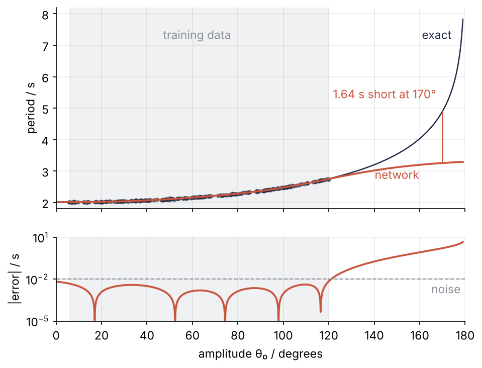
Top: pendulum period in s against amplitude from 0 to 179°. Dots: 200 measurements between 5 and 120°, shaded. Dark line: exact elliptic integral. Red: network, on the curve inside the shaded range and leveling off near 3.3 s beyond it, 1.64 s short at 170°. Bottom: its error in s, crossing the 0.01 s noise level just past 120°.

The top panel shows the measurements, the exact curve, and the network from 0° to 179°, with the range of the training data shaded; the bottom panel shows the network's error on a logarithmic scale. Inside the shaded range the network sits on the curve. Beyond it, the answer is confident and wrong. The six steps below build that figure, from a single gradient to the network's failure.

Setup

PyTorch's CPU build is all this tutorial needs. On Linux the default pip install torch also pulls in the CUDA libraries for NVIDIA graphics cards; the CPU wheel comes from PyTorch's own index:

pip install torch --index-url https://download.pytorch.org/whl/cpu

The two torch settings below make every run give the same numbers to the last digit: deterministic algorithms, and one thread, so that sums are always added up in the same order.

import numpy as np
import torch
import torch.nn as nn
import matplotlib.pyplot as plt
from scipy.special import ellipk

torch.use_deterministic_algorithms(True)
torch.set_num_threads(1)

plt.rcParams.update({
    "figure.figsize": (7, 3.6), "figure.dpi": 110,
    "axes.spines.top": False, "axes.spines.right": False,
    "axes.grid": True, "grid.alpha": 0.25,
    "font.size": 11, "lines.linewidth": 1.8,
})
INK, ACCENT, SECOND, MUTED = "#1f2a44", "#c8553d", "#2a7f9e", "#8a8f98"

g, L = 9.81, 1.0        # m/s^2, m
noise = 0.01            # s, scatter of one timing

def T_exact(deg):
    return 4 * np.sqrt(L / g) * ellipk(np.sin(np.radians(deg) / 2) ** 2)

# the order of these calls fixes every number below
rng = np.random.default_rng(1)
amp = np.sort(rng.uniform(5, 120, 200))                  # degrees
T_meas = T_exact(amp) + rng.normal(0, noise, 200)        # s
perm = rng.permutation(200)
i_train, i_val = perm[:160], perm[160:]

print(f"{len(i_train)} training and {len(i_val)} validation points, "
      f"amplitudes {amp.min():.2f}° to {amp.max():.2f}°, torch {torch.__version__}")

160 training and 40 validation points, amplitudes 5.67° to 119.89°, torch 2.14.1+cpu

Step 1: Make tensors, take a gradient, and step downhill

A tensor is PyTorch's array. You make one from a NumPy array with torch.tensor, and you ask for float32, the precision networks compute in, where NumPy defaults to float64. Before any network, take the simplest model there is, a straight line \(T \approx a + b\,\theta\) with \(\theta\) in radians, fitted to the 160 training points by the mean squared error. Minimization with scipy.optimize.minimize needed the gradient of such a loss; here PyTorch computes it:

theta = torch.tensor(np.radians(amp[i_train]), dtype=torch.float32)
T = torch.tensor(T_meas[i_train], dtype=torch.float32)
print(f"NumPy {amp.dtype}, torch {theta.dtype}")

a = torch.tensor(2.0, requires_grad=True)      # s
b = torch.tensor(0.0, requires_grad=True)      # s per radian
loss = ((a + b * theta - T) ** 2).mean()
loss.backward()

r = (a + b * theta - T).detach()               # the residuals, without the record
print(f"loss = {loss.item():.3f} s²")
print(f"autograd: dloss/da = {a.grad.item():.3f} s,  dloss/db = {b.grad.item():.3f} s")
print(f"by hand:  2 mean(r) = {2 * r.mean().item():.3f} s,  2 mean(r θ) = {2 * (r * theta).mean().item():.3f} s")

NumPy float64, torch torch.float32
loss = 0.104 s²
autograd: dloss/da = -0.484 s,  dloss/db = -0.775 s
by hand:  2 mean(r) = -0.484 s,  2 mean(r θ) = -0.775 s

Because a and b were created with requires_grad=True, PyTorch recorded every operation on them as it ran, and backward() walked that record in reverse with the chain rule. The two gradients agree with the hand formulas, \(r\) being the residual, to the printed digits. That is the gradient minimize needed a hand-written jac for.

Moving downhill is one line per parameter, \(p \leftarrow p - \eta\,\partial(\text{loss})/\partial p\), with a learning rate \(\eta = 0.1\):

lr = 0.1
with torch.no_grad():
    a -= lr * a.grad
    b -= lr * b.grad
    loss = ((a + b * theta - T) ** 2).mean()
print(f"after one step: a = {a.item():.3f} s, b = {b.item():.3f} s, loss = {loss.item():.3f} s²")

after one step: a = 2.048 s, b = 0.078 s, loss = 0.041 s²

The loss falls from 0.104 to 0.041 s². The update sits inside torch.no_grad() because it is not part of the model and must not be recorded; the same block wraps every later evaluation that needs no gradient. Repeat the step and you have gradient descent, which minimize ran for you inside its iterations.

Step 2: Scale inputs and outputs to order one

The network of Step 3 is built from tanh, which changes only for arguments near zero, so it learns fastest when its inputs and outputs are of order one. The amplitudes run to 120° and the periods sit near 2.2 s with a spread of a fifth of a second, so both are standardized: subtract the mean, divide by the standard deviation.

Mean and standard deviation come from the 160 training points only. The 40 validation points stand in for data the network has never seen, so nothing about them may shape the model, and the scaling is part of the model. Computed over all 200 points, it would let the validation set leak into training and make the validation error a less honest test. On your own data the rule is the same: fit the scaling on the training part, then apply those numbers unchanged to everything else, new inputs at prediction time included.

amp_mean, amp_sd = amp[i_train].mean(), amp[i_train].std()
T_mean, T_sd = T_meas[i_train].mean(), T_meas[i_train].std()

def to_tensor(v):
    return torch.tensor(v, dtype=torch.float32)[:, None]    # one row per sample, one column per feature

X_train, X_val = to_tensor((amp[i_train] - amp_mean) / amp_sd), to_tensor((amp[i_val] - amp_mean) / amp_sd)
y_train, y_val = to_tensor((T_meas[i_train] - T_mean) / T_sd), to_tensor((T_meas[i_val] - T_mean) / T_sd)

print(f"θ: mean {amp_mean:.2f}°, sd {amp_sd:.2f}°    T: mean {T_mean:.3f} s, sd {T_sd:.4f} s")
print(f"X_train {tuple(X_train.shape)}, from {X_train.min():.2f} to {X_train.max():.2f}")
print(f"y_train {tuple(y_train.shape)}, from {y_train.min():.2f} to {y_train.max():.2f}")

θ: mean 63.97°, sd 32.95°    T: mean 2.242 s, sd 0.2137 s
X_train (160, 1), from -1.77 to 1.70
y_train (160, 1), from -1.15 to 2.35

The column shape matters because nn.Linear expects one row per sample and one column per feature. Classification with scikit-learn applies the same training-only rule with a scaler object, and the first pitfall below shows what happens without the scaling.

Step 3: Build the network with nn.Sequential

nn.Sequential chains layers, each applied to the output of the one before. nn.Linear(1, 64) turns the one input \(x\) into 64 numbers \(w_i x + b_i\), nn.Tanh() passes each through tanh, and nn.Linear(64, 1) adds them up with weights \(v_i\) and a bias \(c\):

\[\hat y = \sum_{i=1}^{64} v_i \tanh(w_i x + b_i) + c .\]

tanh is a smoothed step from −1 to +1. Each hidden unit is therefore a soft step placed at \(x = -b_i/w_i\), steeper the larger \(w_i\), and flat on both sides of it; the network's curve is a weighted sum of 64 such steps. Those flat sides decide what the network does past its data in Step 6.

def new_model(seed):
    torch.manual_seed(seed)                     # fixes the random starting weights
    return nn.Sequential(nn.Linear(1, 64), nn.Tanh(), nn.Linear(64, 1))

model = new_model(0)
print(model)
print("parameters:", 64 + 64 + 64 + 1, "by hand,", sum(p.numel() for p in model.parameters()), "by numel")

Sequential(
  (0): Linear(in_features=1, out_features=64, bias=True)
  (1): Tanh()
  (2): Linear(in_features=64, out_features=1, bias=True)
)
parameters: 193 by hand, 193 by numel

The first layer has 64 weights and 64 biases, the second 64 weights and one bias. PyTorch draws them uniformly between \(\pm 1/\sqrt{n}\), with \(n\) the number of inputs to the layer, and torch.manual_seed(0) fixes which random numbers, so your run matches this page. Before training, the answers mean nothing, as three validation points show:

with torch.no_grad():
    guess = model(X_val[:3]).numpy()[:, 0] * T_sd + T_mean
for d, Tg, Tm in zip(amp[i_val[:3]], guess, T_meas[i_val[:3]]):
    print(f"{d:6.1f}°   untrained {Tg:.3f} s   measured {Tm:.3f} s")

  75.5°   untrained 2.295 s   measured 2.234 s
  67.5°   untrained 2.313 s   measured 2.199 s
 117.1°   untrained 2.184 s   measured 2.713 s

The untrained network gives a shorter period at 117° than at 67.5°. The curve has no shape yet; training gives it one.

Step 4: Train with a loss, an optimizer, and a loop

The loss, nn.MSELoss(), is the mean squared error of Step 1. The optimizer, torch.optim.Adam(model.parameters(), lr=0.01), holds all 193 parameters, and optimizer.step() does for them what Step 1 did by hand for a and b: it reads each .grad and moves the parameter against it. With torch.optim.SGD that is exactly the update of Step 1. Adam steps along a running average of recent gradients, divided per parameter by a running estimate of their typical size, so steep and shallow directions move at comparable speed. Its learning rate, lr=0.01, is ten times the default, which here needs about six times as many steps to reach the noise. Each of the 3,000 steps uses all 160 training points, a full batch, as Step 1 did.

def train(model, X=X_train, y=y_train, Xv=X_val, yv=y_val, steps=3000, lr=0.01, zero_grad=True):
    loss_fn = nn.MSELoss()
    optimizer = torch.optim.Adam(model.parameters(), lr=lr)
    history = []
    for step in range(steps):
        if zero_grad:
            optimizer.zero_grad()
        loss = loss_fn(model(X), y)
        loss.backward()
        optimizer.step()
        with torch.no_grad():
            val_loss = loss_fn(model(Xv), yv)
        history.append((loss.item(), val_loss.item()))
    return np.sqrt(np.array(history)) * T_sd      # rms in s, training and validation

rms = train(model)
print(" step   training rms   validation rms")
for step in [1, 10, 100, 300, 1000, 3000]:
    print(f"{step:5d}   {rms[step - 1, 0]:9.4f} s   {rms[step - 1, 1]:11.4f} s")

 step   training rms   validation rms
    1      0.2693 s        0.2030 s
   10      0.1280 s        0.1127 s
  100      0.0188 s        0.0162 s
  300      0.0119 s        0.0096 s
 1000      0.0091 s        0.0083 s
 3000      0.0089 s        0.0086 s

optimizer.zero_grad() comes first because backward() adds to .grad instead of overwriting it; the second pitfall shows what that does. The validation loss never calls backward(): it watches the training and must not steer it. The helper converts both losses to rms in seconds, the square root of the MSE times the 0.2137 s of Step 2, and takes model and data as arguments for reuse in Step 6 and the pitfalls. The run takes under two seconds on one CPU core.

Step 5: Read the learning curves

Plot both columns against the step on logarithmic axes and you see the whole training:

steps = np.arange(1, len(rms) + 1)
fig, ax = plt.subplots()
ax.loglog(steps, rms[:, 0], color=INK)
ax.loglog(steps, rms[:, 1], color=ACCENT)
ax.axhline(noise, color=MUTED, ls="--", lw=1)
ax.text(1.2, noise * 1.08, "noise, 0.01 s", color=MUTED, va="bottom")
ax.text(3, rms[2, 0] * 1.15, "training", color=INK)
ax.text(1.5, 0.06, "validation", color=ACCENT, va="top")   # below the dip, clear of both curves
ax.set(xlabel="training step", ylabel="rms error / s", xlim=(1, len(rms)))
plt.show()

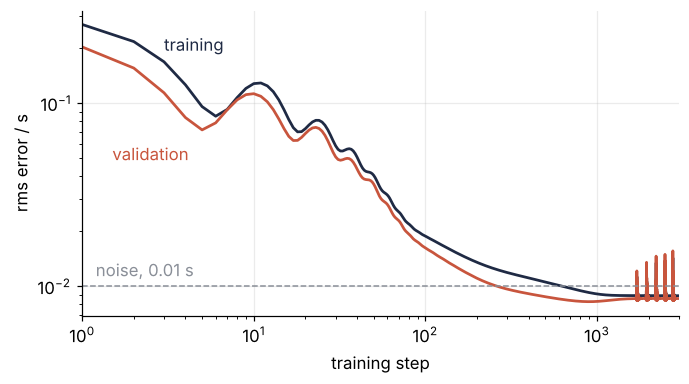
Training and validation rms in s against training step, both axes logarithmic. Dark: training. Red: validation. Both fall from about 0.2 s to the dashed 0.01 s noise level and stay there after about 1,000 steps, apart from a few short spikes.

Both curves fall by a factor of about 20 in the first 300 steps and then lie along the dashed noise line. Four numbers say how closely: when the validation rms first gets below the noise, how often it rises above it later, how far the exact curve itself misses the validation points, and how far the network is from the exact curve.

first = np.argmax(rms[:, 1] < noise) + 1
noise_rms = np.sqrt(np.mean((T_meas[i_val] - T_exact(amp[i_val])) ** 2))
fine = np.linspace(5, 120, 500)
with torch.no_grad():
    T_fine = model(to_tensor((fine - amp_mean) / amp_sd)).numpy()[:, 0] * T_sd + T_mean
print(f"validation rms first below the noise at step {first}")
above = rms[1000:, 1] > noise
print(f"after step 1000: above the noise in {above.sum()} of {above.size} steps, "
      f"highest {rms[1000:, 1].max():.4f} s")
print(f"final rms: training {rms[-1, 0]:.4f} s, validation {rms[-1, 1]:.4f} s")
print(f"exact curve against the validation points: {noise_rms:.4f} s")
print(f"network against the exact curve, 5° to 120°: {np.sqrt(np.mean((T_fine - T_exact(fine)) ** 2)):.4f} s")

validation rms first below the noise at step 263
after step 1000: above the noise in 45 of 2000 steps, highest 0.0156 s
final rms: training 0.0089 s, validation 0.0086 s
exact curve against the validation points: 0.0085 s
network against the exact curve, 5° to 120°: 0.0024 s

The validation rms first drops below the noise at step 263. After step 1,000 the curves are flat except for short spikes up to 0.016 s: one step overshoots, the next overshoots back, and the rms settles within about twenty steps. These spikes are the 45 of the last 2,000 steps above the noise.

The exact curve itself misses the 40 validation points by 0.0085 s, because that is their noise. At the end the network misses them by 0.0086 s: it is as close to them as the true law, and on average no model is closer. Against the exact curve its rms is 0.0024 s, a quarter of the noise. A validation curve that turned up while the training curve kept falling would be overfitting, and the third pitfall shows one.

Step 6: Ask the network beyond its data

To ask the network about any amplitude, scale it with the training numbers of Step 2, evaluate under torch.no_grad(), and scale the answer back:

def predict(model, deg):
    x = to_tensor((np.asarray(deg, dtype=float) - amp_mean) / amp_sd)
    with torch.no_grad():
        return model(x).numpy()[:, 0] * T_sd + T_mean

for d in [30, 120, 140, 150, 170, 179]:
    Tn, Te = predict(model, [d])[0], T_exact(d)
    print(f"{d:4d}°   network {Tn:.3f} s   exact {Te:.3f} s   short by {Te - Tn:6.3f} s ({100 * (Te - Tn) / Te:4.1f} %)")

grid = np.linspace(0, 179, 1791)
err = np.abs(predict(model, grid) - T_exact(grid))
edge = grid[(grid > 120) & (err > noise)][0]
print(f"error first above the noise at {edge:.1f}°")

  30°   network 2.037 s   exact 2.041 s   short by  0.004 s ( 0.2 %)
 120°   network 2.747 s   exact 2.754 s   short by  0.007 s ( 0.3 %)
 140°   network 3.016 s   exact 3.199 s   short by  0.182 s ( 5.7 %)
 150°   network 3.118 s   exact 3.535 s   short by  0.417 s (11.8 %)
 170°   network 3.253 s   exact 4.894 s   short by  1.641 s (33.5 %)
 179°   network 3.291 s   exact 7.826 s   short by  4.535 s (57.9 %)
error first above the noise at 121.1°

Inside the measured range the network is within 0.01 s of the truth. At 140° it is 0.18 s short, at 170° 1.64 s or 34 %, and at 179° 4.53 s. Its error first exceeds the noise at 121.1°, about a degree past the last measurement at 119.9°. The cause is the picture from Step 3: past the last measurement every soft step is on its flat side, so their sum levels off near 3.3 s while the true period runs away. Another seed gives other starting steps, so train five:

T170 = []
for seed in range(5):
    net = new_model(seed)
    train(net)
    T170.append(predict(net, [170])[0])
print("170°:", "  ".join(f"{t:.3f} s" for t in T170), f"   spread {max(T170) - min(T170):.2f} s")

170°: 3.253 s  3.332 s  3.264 s  3.250 s  3.227 s    spread 0.10 s

All five land between 3.23 and 3.33 s, a spread of 0.10 s, and every one is more than 1.5 s short. Agreement between networks is not evidence that they are right outside the data.

T_net = predict(model, grid)
fig, (ax, ax_err) = plt.subplots(2, 1, sharex=True, figsize=(7, 5.4),
                                 gridspec_kw={"height_ratios": [2.4, 1]})
for axis in (ax, ax_err):
    axis.axvspan(amp.min(), amp.max(), color=MUTED, alpha=0.12, lw=0)
ax.plot(amp, T_meas, "o", color=INK, ms=3, alpha=0.6)
ax.plot(grid, T_exact(grid), color=INK, lw=1.2)
ax.plot(grid, T_net, color=ACCENT)
Tn170, Te170 = predict(model, [170])[0], T_exact(170)
ax.plot([170, 170], [Tn170, Te170], color=ACCENT, lw=1.2)
ax.annotate(f"{Te170 - Tn170:.2f} s short at 170°", (170, Te170),
            xytext=(-6, 10), textcoords="offset points", ha="right", va="bottom", color=ACCENT)
ax.text(62, 7.2, "training data", color=MUTED, ha="center")
ax.text(174, 7.2, "exact", color=INK, ha="right")
ax.text(150, 2.75, "network", color=ACCENT, ha="center")
ax.set(ylabel="period / s", ylim=(1.8, 8.2))
ax_err.semilogy(grid, err, color=ACCENT)
ax_err.axhline(noise, color=MUTED, ls="--", lw=1)
ax_err.text(178, noise / 1.6, "noise", color=MUTED, ha="right", va="top")
ax_err.set(xlabel="amplitude θ₀ / degrees", ylabel="|error| / s", xlim=(0, 180), ylim=(1e-5, 10))
plt.show()

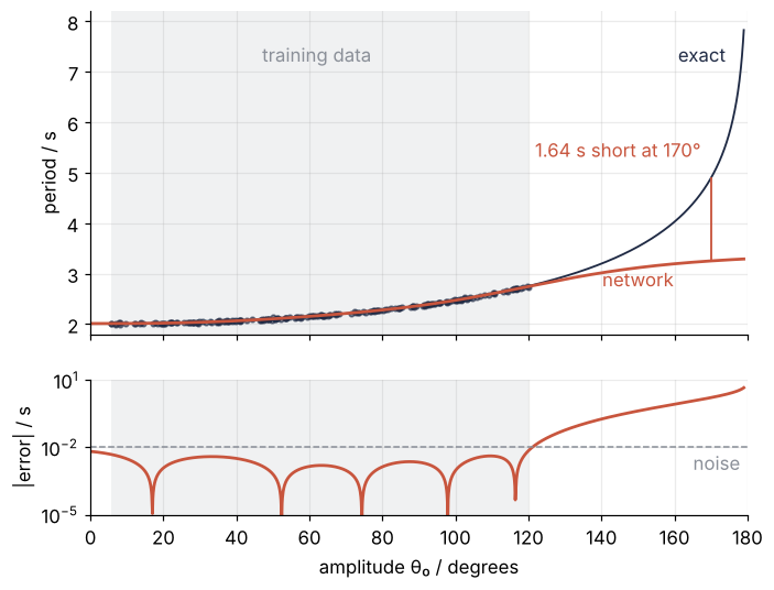
Top: pendulum period in s against amplitude from 0 to 179°. Dots: 200 measurements between 5 and 120°, shaded. Dark line: exact elliptic integral. Red: network, on the curve inside the shaded range and leveling off near 3.3 s beyond it, 1.64 s short at 170°. Bottom: its error in s, crossing the 0.01 s noise level just past 120°.

The 121° edge was found here only because the exact curve is known. On your own problem the range the training data cover stands in for it, and inside that range the validation error of Steps 4 and 5 says how far to trust the network. Outside it nothing in the training says anything.

Pitfalls

Inputs in degrees. Skip Step 2 for the input and feed \(\theta\) in degrees, the output still scaled. Before any training, count the tanh units that are flat over the data, whose output changes by less than 0.1 between 5° and 120°:

W, B = [p.detach().numpy().ravel() for p in new_model(0)[0].parameters()]
for name, (lo, hi) in [("degrees", (5, 120)), ("scaled", ((5 - amp_mean) / amp_sd, (120 - amp_mean) / amp_sd))]:
    flat = np.abs(np.tanh(W * hi + B) - np.tanh(W * lo + B)) < 0.1
    print(f"{name:8s} {flat.sum():2d} of 64 units flat")

rms_deg = train(new_model(0), X=to_tensor(amp[i_train]), Xv=to_tensor(amp[i_val]))
worst = 500 + np.argmax(rms_deg[500:, 1])
print(f"validation rms first below the noise at step {np.argmax(rms_deg[:, 1] < noise) + 1}, "
      f"back up to {rms_deg[worst, 1]:.3f} s at step {worst + 1}")

degrees  44 of 64 units flat
scaled    5 of 64 units flat
validation rms first below the noise at step 1464, back up to 0.094 s at step 1138

With \(x\) in the tens, \(w_i x + b_i\) is far from zero for most units, so they sit on a flat side of their step everywhere the data are. Their gradient is close to zero, and training has to drag them back first: 44 of 64 units are saturated in degrees, against 5 when scaled. The validation rms first drops below the noise at step 1,464 instead of 263 and jumps back to 0.094 s on the way. Adam rescues the run, slowly and erratically. The fix is Step 2.

Forgetting optimizer.zero_grad(). Delete the one line and rerun:

rms_acc = train(new_model(0), zero_grad=False)
for step in [1, 100, 1000, 3000]:
    print(f"{step:5d}   training rms {rms_acc[step - 1, 0]:7.3f} s")

    1   training rms   0.269 s
  100   training rms   1.055 s
 1000   training rms   9.168 s
 3000   training rms  17.098 s

The training rms climbs from 0.27 s to 17 s, for periods that all lie between 2.0 and 2.8 s. backward() adds each new gradient to the old ones, so every step follows the sum of all gradients so far, and that sum keeps pointing where the network was hundreds of steps ago. The fix is the line, first in the loop.

Judging by the training loss alone. A network with many more parameters than data points fits the noise, and its training loss shows it only by being too good. Layers stack the same way as in Step 3: two hidden layers of 256 units, 66,561 parameters, trained with lr 0.001 for 8,000 steps on only the first 20 training points.

torch.manual_seed(0)
wide = nn.Sequential(nn.Linear(1, 256), nn.Tanh(), nn.Linear(256, 256), nn.Tanh(), nn.Linear(256, 1))
rms_wide = train(wide, X=X_train[:20], y=y_train[:20], lr=0.001, steps=8000)
best = np.argmin(rms_wide[:, 1])
print(f"{sum(p.numel() for p in wide.parameters())} parameters")
print(f"best validation rms {rms_wide[best, 1]:.4f} s at step {best + 1}")
print(f"at step 8000: training rms {rms_wide[-1, 0]:.4f} s, validation rms {rms_wide[-1, 1]:.4f} s")

66561 parameters
best validation rms 0.0102 s at step 714
at step 8000: training rms 0.0024 s, validation rms 0.0165 s

The training rms ends at 0.0024 s, four times below the noise, while the validation rms climbs from its best of 0.0102 s at step 714 to 0.0165 s. A training error below the noise level means the network is fitting noise. Watch the validation loss of Step 4, and stop or shrink the network when it turns up.

Variations

A feature that carries the physics. Feed \(\sin(\theta/2)\), or \(-\ln\cos(\theta/2)\), which grows without bound like the period, in place of \(\theta\), and look at the 170° prediction. A tanh network still levels off past its data whatever the input; nn.ReLU(), which is \(\max(0, x)\), in place of nn.Tanh() makes it continue in a straight line instead.
Two inputs. For the period against amplitude and length, use nn.Linear(2, 64) and an input of shape (n, 2), one column per variable, each scaled on its own.
Mini-batches. When the data are too large for one step, wrap them in torch.utils.data.TensorDataset and loop over DataLoader(dataset, batch_size=32, shuffle=True), one optimizer step per batch.
Flux.jl in Julia. The same network is Chain(Dense(1 => 64, tanh), Dense(64 => 1)).

Cheat sheet

X = torch.tensor(x, dtype=torch.float32)[:, None]               # one row per sample; scale with training stats
p = torch.tensor(2.0, requires_grad=True); loss.backward(); p.grad   # autograd
torch.manual_seed(0); torch.use_deterministic_algorithms(True)  # reproducible runs
model = nn.Sequential(nn.Linear(1, 64), nn.Tanh(), nn.Linear(64, 1))
loss_fn = nn.MSELoss()
optimizer = torch.optim.Adam(model.parameters(), lr=1e-2)
optimizer.zero_grad(); loss_fn(model(X), y).backward(); optimizer.step()   # one step, zero_grad first
with torch.no_grad():                                           # validation and prediction: no record
    y_val_pred = model(X_val)