RDKit from the ground up: water solubility from a molecule's structure
Afterwards you can read and draw molecules from SMILES with RDKit, compute descriptors and Morgan fingerprints, and fit models that predict a property.
- Topic
- Machine learning
- Field
- Chemistry
- Prerequisites
- Classification with scikit-learn: telling two populations apart, pandas from the ground up: a week of temperature logs
- Libraries
matplotlib 3.11.2numpy 2.4.3pandas 3.0.6pooch 1.9.0rdkit 2026.9.1sklearn 1.9.1
py-rdkit.ipynb, executed with the versions above. The download needs a free account
Run it yourself. In a terminal, this installs exactly the versions above:
pip install numpy==2.4.3 pooch==1.9.0 rdkit==2026.9.1 pandas==3.0.6 scikit-learn==1.9.1 matplotlib==3.11.2 jupyterlabThe problem: how soluble is a molecule you have only drawn?
Acetamide dissolves in water at logS = +1.58, where logS is the base-10 logarithm of the solubility in mol/L. Decachlorobiphenyl, two benzene rings with every hydrogen replaced by chlorine, sits at −11.6. That is more than 13 log units between two small organic molecules, a factor of 10¹³ in solubility. Suppose all you have is the structure, written as a SMILES string such as CC(=O)N for acetamide. Can you predict logS to within a factor of ten? RDKit, the open-source cheminformatics library for Python, turns that string into a molecule you can compute with.
Delaney answered the question in 2004 with four numbers computed from the structure: the octanol-water partition coefficient cLogP, the molecular weight MW, the number of rotatable bonds RB, and the aromatic proportion AP, the share of heavy atoms that sit in aromatic rings. His fitted equation is
with MW in g/mol. The data are the measured solubilities Delaney compiled (Delaney, J. Chem. Inf. Comput. Sci. 44, 1000, 2004), 1128 compounds in the form the MoleculeNet benchmark distributes them (Wu et al., Chem. Sci. 9, 513, 2018): a CSV file of about 97 KB with one SMILES string and one logS per compound.
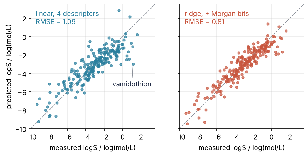
This is where we end up. Each dot is one of 226 molecules held back from fitting, and the closer it sits to the dashed diagonal, the better the prediction. The RMSE is the square root of the mean squared difference between predicted and measured logS, in log units, so an RMSE of 1 means a typical miss by a factor of ten in solubility. It falls from 1.09 for a linear model on Delaney's four descriptors to 0.81 when a Morgan fingerprint of the structure joins them.
Setup
RDKit installs with pip install rdkit and imports as rdkit. The file, MoleculeNet's delaney-processed.csv, 96,699 bytes, comes through pooch.retrieve, which checks its SHA-256 hash and reads it from its cache on later runs. pandas reads it into a DataFrame, and the measured column gets the short name logS.
import warnings
warnings.filterwarnings("ignore", message="IProgress not found")   # from tqdm, which pooch imports

import numpy as np
import pandas as pd
import matplotlib.pyplot as plt
import pooch
import rdkit
from rdkit import Chem, DataStructs, rdBase
from rdkit.Chem import Crippen, Descriptors, Draw, rdFingerprintGenerator
from rdkit.Chem.Scaffolds import MurckoScaffold
from sklearn.model_selection import train_test_split
from sklearn.linear_model import LinearRegression, RidgeCV
from sklearn.preprocessing import StandardScaler
from sklearn.pipeline import make_pipeline
from sklearn.metrics import root_mean_squared_error

plt.rcParams.update({
    "figure.figsize": (7, 3.6), "figure.dpi": 110,
    "axes.spines.top": False, "axes.spines.right": False,
    "axes.grid": True, "grid.alpha": 0.25,
    "font.size": 11, "lines.linewidth": 1.8,
})
INK, ACCENT, SECOND, MUTED = "#1f2a44", "#c8553d", "#2a7f9e", "#8a8f98"
SEED = 0

pooch.get_logger().setLevel("WARNING")
path = pooch.retrieve(
    "https://deepchemdata.s3-us-west-1.amazonaws.com/datasets/delaney-processed.csv",
    known_hash="sha256:8c06a76f0c6487d29ab0f903e6a7a7139f189ab3c1178f159c8be8964602f189")
df = pd.read_csv(path)
df["smiles"] = df["smiles"].str.strip()                 # 212 strings end in a space
df = df.rename(columns={"Compound ID": "name", "measured log solubility in mols per litre": "logS"})
print(f"RDKit {rdkit.__version__}: {len(df)} molecules, logS from {df.logS.min():.2f} to {df.logS.max():.2f}")
RDKit 2026.09.1: 1128 molecules, logS from -11.60 to 1.58
Step 1: Read SMILES into molecules
A SMILES string writes a molecule as one line of text, and five rules cover every string in this tutorial. Atoms are element symbols, and hydrogens are left out: RDKit fills them in from the usual valence. Neighbors in the string are bonded, by a single bond unless = or # marks a double or triple one. Parentheses hold a branch, a digit after an atom opens a ring bond that the same digit closes, and lowercase letters are aromatic atoms. Ethanol is CCO, acetic acid CC(=O)O, benzene c1ccccc1. Caffeine, as the file writes it, has two ring digits, two (=O) branches, and aromatic n and c:
smiles = df.loc[df.name == "Caffeine", "smiles"].item()
caffeine = Chem.MolFromSmiles(smiles)
print(f"{smiles}: {caffeine.GetNumAtoms()} atoms, {caffeine.GetNumBonds()} bonds")
print("canonical:", Chem.MolToSmiles(caffeine))
Cn1cnc2n(C)c(=O)n(C)c(=O)c12: 14 atoms, 15 bonds
canonical: Cn1c(=O)c2c(ncn2C)n(C)c1=O
Chem.MolFromSmiles returns a Mol with 14 atoms, because hydrogens are not counted unless you add them, and 15 bonds, two more than a chain of 14 atoms would have, one per ring. Chem.MolToSmiles writes the canonical SMILES: one string per molecule, whatever order it was written in. Now the whole column:
df["mol"] = [Chem.MolFromSmiles(s) for s in df.smiles]
print(f"not parsed: {df.mol.isna().sum()} of {len(df)}")
not parsed: 0 of 1128
None failed. When RDKit cannot build a molecule, it does not raise an exception: it returns None and writes the reason to its log, which rdBase.CaptureErrorLog catches. Four broken strings, one per rule:
for s in ["CC(C", "C1CC", "CC(C)(C)(C)C", "c1cccc1"]:
    with rdBase.CaptureErrorLog() as log:
        m = Chem.MolFromSmiles(s)
    reason = log.messages.splitlines()[0].partition("] ")[2]   # cut the time stamp
    print(f"{s:14s} {m}  {reason}")
CC(C           None  SMILES Parse Error: extra open parentheses while parsing: CC(C
C1CC           None  SMILES Parse Error: unclosed ring for input: 'C1CC'
CC(C)(C)(C)C   None  Explicit valence for atom # 1 C, 5, is greater than permitted
c1cccc1        None  Can't kekulize mol.  Unkekulized atoms: 0 1 2 3 4
The first two fail in the parser: a branch never closed, ring 1 opened and never closed. The other two parse and then fail sanitization, the check RDKit runs on every new molecule: it checks valences, perceives aromaticity, and assigns a Kekulé structure of alternating single and double bonds. A carbon with five bonds fails the first test, and five aromatic carbons fit no alternating pattern. Canonical strings also find repeats:
df["canonical"] = [Chem.MolToSmiles(m) for m in df.mol]
print(f"{df.canonical.duplicated().sum()} molecules repeat an earlier one")
11 molecules repeat an earlier one
The file holds 11 molecules twice. Duplicates matter when the data are split, as Pitfalls shows.
Step 2: Draw molecules and look at their atoms
Draw.MolsToGridImage draws a list of molecules side by side. Here are the most soluble molecule in the file, caffeine, testosterone, and the least soluble:
picks = [df.logS.idxmax(), df.index[df.name == "Caffeine"][0],
         df.index[df.name == "Testosterone"][0], df.logS.idxmin()]
names = {df.name[picks[-1]]: "Decachlorobiphenyl"}      # the file calls it 2,2',3,3',4,4',5,5',6,6'-PCB
opts = Draw.MolDrawOptions()
opts.legendFontSize = 18                                # one size for every legend
Draw.MolsToGridImage(list(df.mol[picks]), molsPerRow=2, subImgSize=(380, 240), drawOptions=opts,
                     legends=[f"{names.get(df.name[i], df.name[i])}, logS = {df.logS[i]:.2f}" for i in picks])
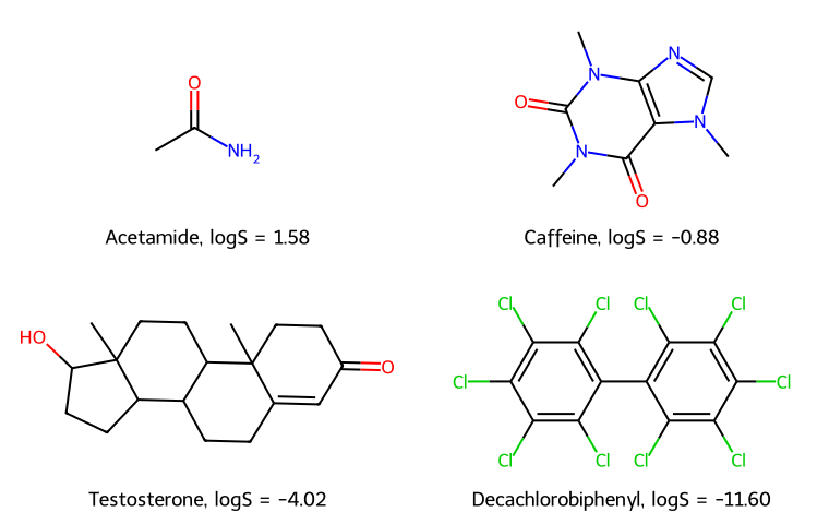
legends puts a line of text under each drawing, molsPerRow sets the grid, and drawOptions carries settings such as the legend font size; the call returns an image, which the notebook shows. In reading order the molecules grow larger and greasier, and logS falls by 13 units. A Mol also hands you its atoms:
aromatic = [a.GetSymbol() for a in caffeine.GetAtoms() if a.GetIsAromatic()]
print(f"{len(aromatic)} of {caffeine.GetNumHeavyAtoms()} heavy atoms aromatic: {' '.join(aromatic)}")
9 of 14 heavy atoms aromatic: N C N C N C N C C
Nine of caffeine's 14 heavy atoms are aromatic, every atom of both rings. RDKit's aromaticity model counts the six-membered ring with its two C=O groups as aromatic too, which is why the canonical SMILES of Step 1 writes it in lowercase. That share is Delaney's aromatic proportion.
Step 3: Compute Delaney's four descriptors
Three of the descriptors are one function call each. Crippen.MolLogP estimates cLogP by summing contributions of atom types (the method of Wildman and Crippen), which is not the Daylight ClogP program Delaney used. Descriptors.MolWt and Descriptors.NumRotatableBonds compute what their names say, and the aromatic proportion is the short function you could write after Step 2:
def aromatic_proportion(m):
    return sum(a.GetIsAromatic() for a in m.GetAtoms()) / m.GetNumHeavyAtoms()

desc = pd.DataFrame({
    "cLogP": df.mol.map(Crippen.MolLogP),
    "MW": df.mol.map(Descriptors.MolWt),
    "RB": df.mol.map(Descriptors.NumRotatableBonds),
    "AP": df.mol.map(aromatic_proportion),
})
desc.describe().round(2)
| cLogP | MW | RB | AP | |
|---|---|---|---|---|
| count | 1128.00 | 1128.00 | 1128.00 | 1128.00 |
| mean | 2.45 | 203.94 | 2.18 | 0.36 |
| std | 1.85 | 102.74 | 2.64 | 0.34 |
| min | -7.57 | 16.04 | 0.00 | 0.00 |
| 25% | 1.41 | 121.18 | 0.00 | 0.00 |
| 50% | 2.34 | 182.18 | 1.00 | 0.38 |
| 75% | 3.40 | 270.37 | 3.00 | 0.67 |
| max | 10.39 | 780.95 | 23.00 | 1.00 |
The scales differ: the molecular weight has a standard deviation of 102.74 g/mol, the other three between 0.34 and 2.64. Step 5 has to deal with that. Two of the four can be checked against columns the file ships with:
print(f"largest MW difference to the file: {np.abs(desc.MW - df['Molecular Weight']).max():.0e} g/mol")
print(f"rows where RB differs from the file: {(desc.RB != df['Number of Rotatable Bonds']).sum()}")
largest MW difference to the file: 6e-14 g/mol
rows where RB differs from the file: 0
A difference of 6e-14 g/mol is rounding, and the rotatable bonds agree in every row. cLogP has no column to check against, so Crippen's you take on trust.
Step 4: Fit a linear model and compare with Delaney's equation
Split the row indices, not the descriptor table, so that the fingerprints of Step 5 get the same 226 test molecules. The split and .fit work as in the scikit-learn tutorial, Step 1:
train, test = train_test_split(np.arange(len(df)), test_size=0.2, random_state=SEED)
X, y = desc.to_numpy(), df.logS.to_numpy()
lin = LinearRegression().fit(X[train], y[train])

delaney = {"intercept": 0.16, "cLogP": -0.63, "MW": -0.0062, "RB": 0.066, "AP": -0.74}
print(f"{len(train)} training, {len(test)} test molecules\n")
print(f"{'':10s}{'refit':>9s}{'Delaney':>9s}")
for name, refit in zip(delaney, [lin.intercept_, *lin.coef_]):
    print(f"{name:10s}{refit:9.4f}{delaney[name]:9.4f}")
902 training, 226 test molecules

              refit  Delaney
intercept    0.1961   0.1600
cLogP       -0.7534  -0.6300
MW          -0.0064  -0.0062
RB           0.0189   0.0660
AP          -0.4201  -0.7400
MW agrees with Delaney to about 3 % (−0.0064 against −0.0062), while the refit steepens cLogP from −0.63 to −0.75 and shrinks the aromatic and rotatable-bond terms. Two reasons, which this data set cannot separate: RDKit's cLogP is not Delaney's, and he fitted a larger set of 2874 compounds. The test is what counts, three sets of predictions for the same 226 molecules:
def rmse(pred):
    return root_mean_squared_error(y[test], pred)

b = np.array(list(delaney.values()))
esol = df["ESOL predicted log solubility in mols per litre"].to_numpy()
print(f"refit on RDKit descriptors:            RMSE {rmse(lin.predict(X[test])):.2f}")
print(f"Delaney's coefficients, RDKit descr.:  RMSE {rmse(b[0] + X[test] @ b[1:]):.2f}")
print(f"Delaney's own predictions (the file):  RMSE {rmse(esol[test]):.2f}")
refit on RDKit descriptors:            RMSE 1.09
Delaney's coefficients, RDKit descr.:  RMSE 1.19
Delaney's own predictions (the file):  RMSE 0.94
The refit misses by 1.09 log units, Delaney's coefficients on RDKit's descriptors by 1.19, and Delaney's own predictions, made with his own descriptors, by 0.94. The published equation does best with the descriptors it was fitted on. A set of coefficients does not travel between descriptor implementations.
Step 5: Add Morgan fingerprints
Four numbers do not say which groups a molecule carries. A Morgan fingerprint does. For every atom, RDKit takes up to three neighborhoods: the atom alone, the atom with its neighbors one bond away, and out to two bonds, the radius. Each is hashed to an integer whose remainder modulo 2048 picks one of 2048 bits; a bit is on if any neighborhood lands there. Identical neighborhoods share a bit, and so can different ones, the price of a fixed length:
gen = rdFingerprintGenerator.GetMorganGenerator(radius=2, fpSize=2048)
fps = np.array([gen.GetFingerprintAsNumPy(m) for m in df.mol])
print(f"fingerprints {fps.shape}, caffeine {gen.GetFingerprintAsNumPy(caffeine).sum()} bits on, "
      f"mean {fps.sum(axis=1).mean():.1f}")
fingerprints (1128, 2048), caffeine 25 bits on, mean 21.5
Caffeine sets 25 of the 2048 bits, more than its 14 atoms because each atom contributes up to three neighborhoods, and the average molecule sets 21.5. With 2052 columns for 902 molecules, least squares would fit the noise. Ridge regression adds a penalty on coefficient size, and RidgeCV picks its strength alpha by cross-validation.
A penalty on coefficient size makes a column's units decide how hard it is penalized, so the four descriptors are standardized, as in the scikit-learn tutorial, Step 5. The bits are not: they already share one scale. Standardizing divides by the standard deviation, small for a rare bit, and the cell prints it for one on in three of 902 molecules before standardizing everything anyway:
p = 3 / len(train)                                       # a bit on in 3 training molecules
print(f"standard deviation of a bit on in 3 of {len(train)}: {np.sqrt(p * (1 - p)):.3f}")
alphas = np.logspace(-1, 4, 21)
X_all = np.hstack([X, fps])
everything = make_pipeline(StandardScaler(), RidgeCV(alphas=alphas)).fit(X_all[train], y[train])
print(f"all 2052 columns standardized:         RMSE {rmse(everything.predict(X_all[test])):.2f}")

scaler = StandardScaler().fit(X[train])                 # descriptors only; the bits stay 0 and 1
Z = np.hstack([scaler.transform(X), fps])
ridge = RidgeCV(alphas=alphas).fit(Z[train], y[train])
print(f"descriptors standardized, bits as is:  RMSE {rmse(ridge.predict(Z[test])):.2f}, alpha = {ridge.alpha_:.1f}")
bits = RidgeCV(alphas=alphas).fit(fps[train], y[train])
print(f"fingerprint alone:                     RMSE {rmse(bits.predict(fps[test])):.2f}")
standard deviation of a bit on in 3 of 902: 0.058
all 2052 columns standardized:         RMSE 1.07
descriptors standardized, bits as is:  RMSE 0.81, alpha = 10.0
fingerprint alone:                     RMSE 1.22
Dividing by 0.058 makes that bit 17 times larger, so a coefficient 17 times smaller has the same effect and pays far less penalty: the rarest, noisiest bits go nearly unrestrained. Standardizing everything gives 1.07, hardly better than the linear model's 1.09. With the bits left alone the model reaches 0.81, at alpha = 10.0. The fingerprint alone gives 1.22, worse than four descriptors: a bit records that a neighborhood occurs, not how often, so 1-hexanol and 1-octadecanol look the same to it, as Pitfalls shows. The two kinds of columns carry different information, and the model needs both.
Step 6: Plot predicted against measured solubility
The last step puts both models' test predictions against the measurements, with the RMSE written into each panel:
models = [("linear, 4 descriptors", lin.predict(X[test]), SECOND),
          ("ridge, + Morgan bits", ridge.predict(Z[test]), ACCENT)]
lim = (-10, 3.5)
fig, axes = plt.subplots(1, 2, figsize=(8, 4.2), sharex=True, sharey=True)
for ax, (label, pred, color) in zip(axes, models):
    ax.plot(lim, lim, ls="--", lw=1, color=MUTED)
    ax.plot(y[test], pred, "o", ms=4, alpha=0.7, color=color)
    ax.text(0.04, 0.96, f"{label}\nRMSE = {rmse(pred):.2f}", transform=ax.transAxes,
            va="top", color=color)
    ax.set(xlabel="measured logS / log(mol/L)", xlim=lim, ylim=lim,
           xticks=range(-10, 3, 2), yticks=range(-10, 3, 2), aspect="equal")
axes[0].set_ylabel("predicted logS / log(mol/L)")
err = np.abs(models[0][1] - y[test])
w = err.argmax()                                         # the linear model's largest miss
axes[0].annotate(df.name[test[w]], (y[test][w], models[0][1][w]), xytext=(1.0, -4.7),
                 ha="center", va="top", color=INK, arrowprops=dict(arrowstyle="-", lw=1, color=MUTED))
plt.show()

top = y[test] > -1                                       # the most soluble test molecules
for label, pred, _ in models:
    print(f"{label:22s} mean error for {top.sum()} molecules above logS = -1: {np.mean(pred[top] - y[test][top]):+.2f}")
print(f"largest linear error: {err[w]:.2f} log units ({df.name[test[w]]})")
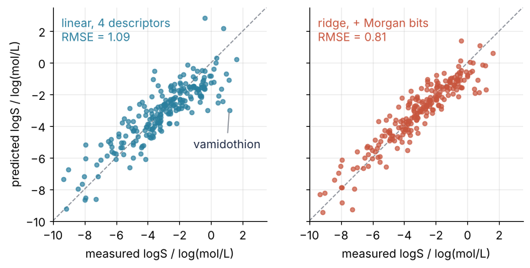
linear, 4 descriptors  mean error for 43 molecules above logS = -1: -1.07
ridge, + Morgan bits   mean error for 43 molecules above logS = -1: -0.71
largest linear error: 4.13 log units (vamidothion)
Both clouds follow the diagonal, the ridge cloud more tightly. The linear cloud runs flatter than the diagonal: it puts the 43 most soluble molecules too low by 1.07 log units on average, where ridge misses them by 0.71. The largest linear miss, 4.13 log units, is vamidothion, an insecticide that dissolves far better than its four descriptors predict.
Pitfalls
SMILES that fail silently. A list comprehension with if m is not None drops the failures without a word. The molecule list is then shorter than the logS column, every molecule from the first failure on is paired with its neighbor's solubility, and the model fits the shifted data without an error. Or a None survives until Crippen.MolLogP(None) raises, three cells away from the string that caused it. Keep the molecules in a DataFrame column, as Step 1 does, and drop whole rows with df.dropna(subset=["mol"]), never entries of a list.
A random split with near-identical molecules on both sides. The test RMSE flatters the model for new chemistry. Tanimoto similarity measures how alike two fingerprints are: the number of bits on in both, divided by the number on in either, 1 for identical fingerprints and 0 for none in common. DataStructs computes it on RDKit's own bit vectors, from gen.GetFingerprint, not on NumPy arrays. Take each test molecule's highest similarity to the training set:
bitvects = [gen.GetFingerprint(m) for m in df.mol]
train_fps = [bitvects[j] for j in train]
nearest = np.array([max(DataStructs.BulkTanimotoSimilarity(bitvects[i], train_fps)) for i in test])
same = test[nearest == 1]
dup = df.canonical[same].isin(set(df.canonical[train])).sum()
print(f"identical fingerprint in training: {len(same)} of {len(test)} ({dup} the same molecule)")
print(f"neighbor at 0.8 or above: {(nearest >= 0.8).sum()}, median of the highest: {np.median(nearest):.2f}")
octanol = df.index[df.name == "1-Octanol"][0]
print(f"same fingerprint as 1-octanol (logS {df.logS[octanol]:.2f}):",
      ", ".join(f"{df.name[j]} ({df.logS[j]:.2f})" for j in train if bitvects[j] == bitvects[octanol]))
identical fingerprint in training: 13 of 226 (1 the same molecule)
neighbor at 0.8 or above: 23, median of the highest: 0.56
same fingerprint as 1-octanol (logS -2.39): 1-Dodecanol (-4.80), 1-Octadecanol (-8.40), 1-Decanol (-3.63), 1-Heptanol (-1.81), 1-Hexanol (-1.24)
Thirteen test molecules have an identical fingerprint in training and 23 a neighbor at 0.8 or above, where the median is 0.56. Only one of the 13 is one of Step 1's repeats. The other 12 are different molecules that radius 2 cannot tell apart: 1-octanol, at logS = −2.39, shares its fingerprint with five training alcohols that span −1.24 for 1-hexanol to −8.40 for 1-octadecanol. A scaffold split asks the harder question. The Bemis-Murcko scaffold is what is left of a molecule once every side chain is cut away, its rings and the chains that link them. The split keeps all molecules on one scaffold on the same side: the largest scaffold groups fill the training set up to 80 % of the molecules, and the rest go to test. Rare scaffolds land there, so the test set is chemistry the model has not seen:
scaffold = df.mol.map(lambda m: MurckoScaffold.MurckoScaffoldSmiles(mol=m))
groups = sorted(df.groupby(scaffold).groups.items(), key=lambda g: (-len(g[1]), g[0]))
train_s, test_s = [], []
for scaf, rows in groups:                                # largest scaffold groups go to training
    (train_s if len(train_s) + len(rows) <= 0.8 * len(df) else test_s).extend(rows)
train_s, test_s = np.array(train_s), np.array(test_s)
print(f"{len(train_s)} training, {len(test_s)} test, {(scaffold[train_s] == '').sum()} acyclic in training")

lin_s = LinearRegression().fit(X[train_s], y[train_s])
Z_s = np.hstack([StandardScaler().fit(X[train_s]).transform(X), fps])
ridge_s = RidgeCV(alphas=alphas).fit(Z_s[train_s], y[train_s])
print(f"linear RMSE {root_mean_squared_error(y[test_s], lin_s.predict(X[test_s])):.2f}, "
      f"ridge RMSE {root_mean_squared_error(y[test_s], ridge_s.predict(Z_s[test_s])):.2f}")
902 training, 226 test, 317 acyclic in training
linear RMSE 1.34, ridge RMSE 1.13
The 317 acyclic molecules share the empty scaffold and go to training as the largest group. On new scaffolds the linear RMSE rises from 1.09 to 1.34 and the ridge RMSE from 0.81 to 1.13. When the model is meant for new chemistry, report the scaffold split.
Comparing an RMSE with a published one. Your 0.81 beats a paper's number, or loses to it, and either way that means little. Another split, test size, or descriptor set moves an RMSE as much as a better method does; Step 4 showed what other descriptors do to the same equation. The split alone:
for seed in range(5):
    tr, te = train_test_split(np.arange(len(df)), test_size=0.2, random_state=seed)
    Zs = np.hstack([StandardScaler().fit(X[tr]).transform(X), fps])
    l = root_mean_squared_error(y[te], LinearRegression().fit(X[tr], y[tr]).predict(X[te]))
    r = root_mean_squared_error(y[te], RidgeCV(alphas=alphas).fit(Zs[tr], y[tr]).predict(Zs[te]))
    print(f"seed {seed}: linear {l:.2f}, ridge {r:.2f}")
seed 0: linear 1.09, ridge 0.81
seed 1: linear 1.00, ridge 0.79
seed 2: linear 0.98, ridge 0.81
seed 3: linear 1.01, ridge 0.78
seed 4: linear 0.93, ridge 0.75
Five seeds give linear RMSEs from 0.93 to 1.09 and ridge RMSEs from 0.75 to 0.81, and seed 0, fixed before looking, sits at the top of both ranges. Compute the reference on your own split and quote the split with the number.
Variations
- Substructure search. SMARTS is SMILES extended with queries, a pattern language for parts of molecules.
pattern = Chem.MolFromSmarts("cCl")matches a chlorine on an aromatic carbon, anddf.mol.map(lambda m: m.HasSubstructMatch(pattern))selects the molecules that carry one, so you can score the model on chlorinated aromatics alone. - Similarity search.
DataStructs.BulkTanimotoSimilarity(query, bitvects)scores one fingerprint against all 1128; sort, keep the five highest, and draw them withMolsToGridImage. - Another MoleculeNet property. FreeSolv (hydration free energies) and Lipophilicity (octanol-water distribution coefficients) come as CSV files with a SMILES column; change the file and the target column.
- Count fingerprints or a nonlinear model.
gen.GetCountFingerprintAsNumPy(m)counts how often each neighborhood occurs instead of flagging it, andRandomForestRegressorfromsklearn.ensemblereplaces ridge. Fit the forest on the four descriptors alone first: on this split that already matches the ridge model, so any gain belongs to the nonlinearity, not the fingerprint.
Cheat sheet
m = Chem.MolFromSmiles(s)                     # None on failure, no exception
with rdBase.CaptureErrorLog() as log: m = Chem.MolFromSmiles(s)   # log.messages holds the reason
Chem.MolToSmiles(m)                           # canonical: one string per molecule
Draw.MolsToGridImage(mols, molsPerRow=4, legends=names)
Crippen.MolLogP(m), Descriptors.MolWt(m), Descriptors.NumRotatableBonds(m)
gen = rdFingerprintGenerator.GetMorganGenerator(radius=2, fpSize=2048)
gen.GetFingerprintAsNumPy(m)                  # 0/1 array for scikit-learn; gen.GetFingerprint(m) for RDKit
DataStructs.BulkTanimotoSimilarity(fp, fps)   # one fingerprint against a list
MurckoScaffold.MurckoScaffoldSmiles(mol=m)    # rings and their linkers; "" if acyclic
StandardScaler().fit(X_desc[train])           # descriptors only, never the bits
Further reading
- RDKit, Getting Started with the RDKit in Python, and the
rdFingerprintGeneratorreference. - The OpenSMILES specification, for the parts of the grammar Step 1 leaves out: brackets, charges, isotopes, and stereochemistry.
- Delaney, "ESOL: estimating aqueous solubility directly from molecular structure", J. Chem. Inf. Comput. Sci. 44, 1000 (2004), doi:10.1021/ci034243x; Wu et al., "MoleculeNet: a benchmark for molecular machine learning", Chem. Sci. 9, 513 (2018), doi:10.1039/C7SC02664A.
- Leach and Gillet, An Introduction to Chemoinformatics (Springer, revised edition 2007), for descriptors and similarity searching.
- Related tutorials on this site: Classification with scikit-learn: telling two populations apart for splits and pipelines; Overfitting: why the model that fits its data best predicts worst; PCA with scikit-learn: sixty absorption spectra in two dimensions, another chemistry data set; pandas from the ground up: a week of temperature logs.
- Download the notebook. It was executed with the library versions in the header.