Nonlinear systems with scipy.optimize.root: three steady states of a reactor

The problem: one reactor, three steady states

An exothermic reaction A → B runs in a stirred tank that is cooled through a jacket. Feed and jacket are at 298 K. With the same feed and cooling, this reactor can run steadily at 311 K or at 368 K, 57 K apart, depending on how it was started. Finding these states means solving a nonlinear system of two equations in two unknowns, which is the job of scipy.optimize.root.

The unknowns are the conversion \(X\), the fraction of A that has reacted, and the temperature \(T\). Feed flows through at one reactor volume per hour, so the residence time \(V/F\) is 1 h. At steady state, what flows in minus what flows out minus what reacts is zero, for A and for heat, per m³ of reactor:

with the Arrhenius rate constant \(k(T) = k_0\,e^{-E/RT}\). Here \(C_{Af}\) is the feed concentration of A, \(T_f\) and \(T_j\) the feed and jacket temperatures, \(-\Delta H\) the heat of reaction, \(\rho c_p\) the heat capacity per volume, and \(UA/V\) the cooling coefficient. The mass balance gives \(X\) in terms of \(T\), but the energy balance left over has no closed-form solution for \(T\). The parameters are Case 2 of the exothermic CSTR in Bequette's Process Dynamics (1998), Module 9, Table M9.1. Van Heerden (1953) explained the three states as crossings of an S-shaped heat-generation curve with a straight heat-removal line.

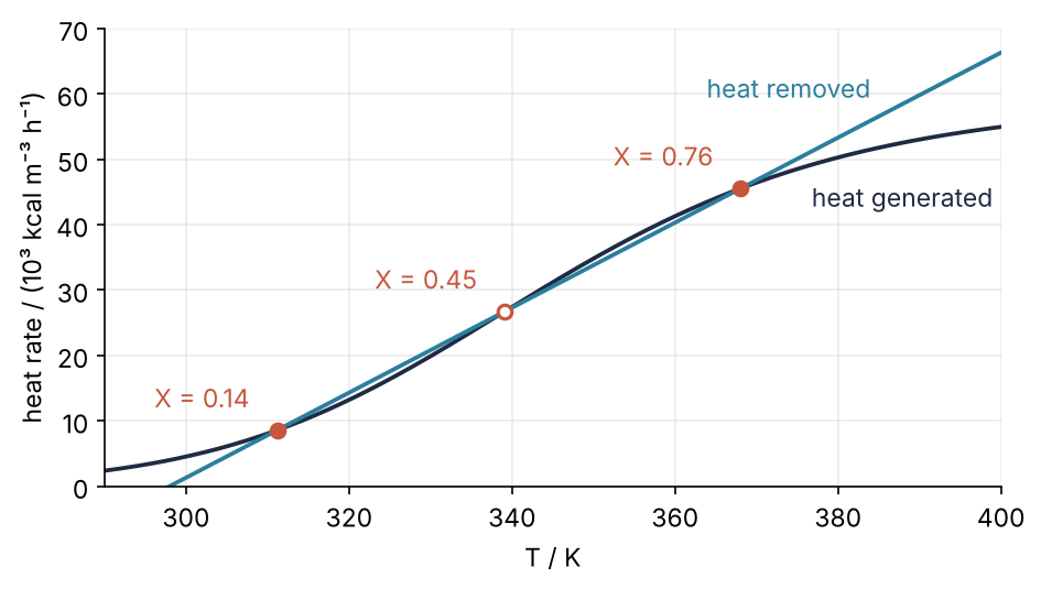
The markers are what root finds from a grid of starts in Step 5, and Step 6 draws the curves.

Setup

The units are the textbook's: kcal, kmol, m³, h, and K.

import warnings

import numpy as np
import matplotlib.pyplot as plt
from scipy.optimize import root, fsolve, approx_fprime, least_squares

F_V = 1.0           # F/V, 1/h
k0 = 9703 * 3600    # 1/h
E = 11843.0         # kcal/kmol
R = 1.987           # kcal/(kmol K)
dH = 5960.0         # -ΔH, kcal/kmol
rhoCp = 500.0       # kcal/(m^3 K)
CAf = 10.0          # kmol/m^3
Tf = 298.0          # K
Tj = 298.0          # K
UA_V = 150.0        # kcal/(m^3 h K)

def k(T):
    return k0 * np.exp(-E / (R * T))

plt.rcParams.update({
    "figure.figsize": (7, 3.6), "figure.dpi": 110,
    "axes.spines.top": False, "axes.spines.right": False,
    "axes.grid": True, "grid.alpha": 0.25,
    "font.size": 11, "lines.linewidth": 1.8,
})
INK, ACCENT, SECOND, MUTED = "#1f2a44", "#c8553d", "#2a7f9e", "#8a8f98"

dT_ad = dH * CAf / rhoCp
print(f"adiabatic temperature rise {dT_ad:.1f} K, so no steady state is above {Tf + dT_ad:.0f} K")

adiabatic temperature rise 119.2 K, so no steady state is above 417 K

Without any cooling, a feed that reacted completely would heat itself by 119.2 K. With cooling, every steady state is colder than 417 K, a limit Step 5 uses.

Step 1: Write both balances as one residual function

root wants a single function that takes the vector of unknowns and returns a vector of the same length, zero at a solution. Each entry is called a residual: what is left of a balance that does not yet hold. Call the unknowns \(u = (X, T)\) and the residuals \(f(u)\).

def residual(u):
    X, T = u
    reacted = k(T) * CAf * (1 - X)
    mass = -F_V * CAf * X + reacted
    energy = rhoCp * F_V * (Tf - T) + dH * reacted + UA_V * (Tj - T)
    return np.array([mass, energy])

print(residual((0.0, 298.0)))
print(residual((0.5, 340.0)))

[7.19394045e-01 4.28758851e+03]
[-7.44572757e-01 -1.93765363e+03]

Both rows change sign between the two points. For one unknown that would trap a root. For two it only means that each balance holds somewhere on the segment between them, not both at the same point.

The first row is in kmol/(m³ h), the second in kcal/(m³ h), and they differ by a factor of about 10⁴. A residual of 0.001 would be a poor mass balance and a perfect energy balance. So a residual means nothing until each row is compared with the size of its own terms. A good scale for a row is its largest term at ordinary conditions: here the flow of A coming in with the feed, \((F/V)\,C_{Af}\), and the enthalpy the feed carries in, \(\rho c_p (F/V)\,T_f\).

scale = np.array([F_V * CAf, rhoCp * F_V * Tf])

def scaled_residual(u):
    return residual(u) / scale

print(scale)

[1.00e+01 1.49e+05]

The scaled residual is dimensionless. A value of 1e-8 means that the balance holds to eight digits of its own feed term, and that is the test Step 5 applies.

Step 2: Solve from one start and read the result

Start at the feed state, no conversion and room temperature, and print everything that comes back:

res = root(residual, (0.0, 300.0))
print(res)

 message: The solution converged.
 success: True
  status: 1
     fun: [ 2.587e-13  1.545e-09]
       x: [ 1.436e-01  3.112e+02]
  method: hybr
    nfev: 11
    fjac: [[-2.380e-03 -1.000e+00]
           [ 1.000e+00 -2.380e-03]]
       r: [ 4.519e+03  1.828e+02  5.134e-01]
     qtf: [-1.008e-04 -2.230e-07]

The default method, hybr, is Newton's idea carried to two unknowns. For one equation, as in Root finding with scipy.optimize, Newton replaces the curve by its tangent at the current guess and jumps to where the tangent crosses zero. For two unknowns the tangent becomes a table of slopes, the Jacobian \(J\): a 2 × 2 matrix whose entry in row \(i\) and column \(j\) says how much residual \(i\) changes when unknown \(j\) moves a little. Its first row holds \(\partial\,\text{mass}/\partial X\) and \(\partial\,\text{mass}/\partial T\), its second row the same for the energy balance. Each step solves \(J\,\Delta u = -f(u)\) for the correction \(\Delta u\) and repeats.

hybr is MINPACK's modification of Powell's hybrid method, which bends that step toward the steepest descent of the sum of squared residuals when the full step would go too far. It computes \(J\) once by finite differences, one extra residual call per unknown, and afterwards usually updates it from how \(f\) changed between guesses.

x is the answer, a conversion of 0.1436 at 311.17 K, after 11 calls of residual (nfev). success and message report convergence. fjac, r, and qtf are MINPACK's working matrices (the QR factors of the last approximate Jacobian, and \(Q^\mathsf{T}\) times fun), and you can skip them. Read fun against the scales of Step 1, not as raw numbers: 1.5e-9 kcal/(m³ h) is a scaled residual of 1e-14.

Step 3: Start somewhere else

Start hot and fully converted, then halfway:

for x0 in [(1.0, 400.0), (0.5, 340.0)]:
    r = root(residual, x0)
    print(f"start X = {x0[0]:.1f}, T = {x0[1]:.0f} K  ->  X = {r.x[0]:.4f}, T = {r.x[1]:.2f} K, nfev = {r.nfev}")

start X = 1.0, T = 400 K  ->  X = 0.7641, T = 368.06 K, nfev = 15
start X = 0.5, T = 340 K  ->  X = 0.4482, T = 339.10 K, nfev = 11

The hot state at 368.06 K, and a third one at 339.10 K. The same equations have three answers, and the start decides which one you get. No single call tells you how many there are.

Step 4: Supply the Jacobian

The four slopes are short to write down, because \(dk/dT = k\,E/(RT^2)\):

A wrong Jacobian is worse than none, so check it first. approx_fprime takes a vector function and returns its finite-difference Jacobian:

def jacobian(u):
    X, T = u
    kT = k(T)
    dk = kT * E / (R * T**2)
    return np.array([
        [-F_V * CAf - kT * CAf, dk * CAf * (1 - X)],
        [-dH * kT * CAf, -rhoCp * F_V - UA_V + dH * dk * CAf * (1 - X)],
    ])

u = np.array([0.3, 330.0])
J_exact, J_fd = jacobian(u), approx_fprime(u, residual)
print(f"largest relative difference {np.max(np.abs(J_fd - J_exact) / np.abs(J_exact)):.1e}")

res = root(residual, (0.0, 300.0), jac=jacobian)
print(f"X = {res.x[0]:.4f}, T = {res.x[1]:.2f} K, nfev = {res.nfev}, njev = {res.njev}")

largest relative difference 2.5e-06
X = 0.1436, T = 311.17 K, nfev = 9, njev = 1

The two agree to 2.5e-6, about what a forward difference can resolve, so the algebra is right. With it root needs 9 residual calls and one Jacobian, against 11 calls before. The two calls saved are the one finite-difference Jacobian of Step 2, one call per unknown. The saving grows with the number of unknowns and with the cost of one residual. For two unknowns, writing \(J\) is a check on your understanding more than a speedup.

Step 5: Find all three from a grid of starts

Since the start decides the answer, start from many places. That takes four choices, which carry over to any system: the box, the filter, and the tolerance before the run, the density after it.

The box. Each unknown runs between its physical limits: \(0 \le X \le 1\), and \(T\) from just below 298 K to the adiabatic limit of 417 K from Setup. No steady state is colder than 298 K, because feed and jacket are both at 298 K and the reaction only releases heat. The grid covers 290 to 410 K.

The filter. Keep a solution only if success is True and every scaled residual is below 1e-8. success alone is not enough: it reports that the steps became small, not that the balances hold, as the first pitfall shows.

The tolerance. Sort by \(T\) and start a new group wherever neighbors differ by more than 0.1 K. The run below checks that choice.

def find_all(X0s, T0s):
    found, failed = [], 0
    for X0 in X0s:
        for T0 in T0s:
            r = root(residual, (X0, T0), jac=jacobian)
            if r.success and np.all(np.abs(r.fun / scale) < 1e-8):
                found.append(r.x)
            else:
                failed += 1
    found = np.array(sorted(found, key=lambda x: x[1]))
    groups = np.split(found, np.nonzero(np.diff(found[:, 1]) > 0.1)[0] + 1)
    return groups, failed

groups, failed = find_all(np.linspace(0, 1, 11), np.arange(290, 411, 10))
states = np.array([g.mean(axis=0) for g in groups])
print(f"{sum(map(len, groups))} kept, {failed} failed")
print(" starts      X    T / K   C_A / (kmol/m^3)   spread / K")
for g, (X, T) in zip(groups, states):
    print(f"{len(g):6d}  {X:.4f}  {T:7.3f}  {CAf * (1 - X):10.3f}  {np.ptp(g[:, 1]):17.1e}")
print("distance between neighbors / K:", np.round(np.diff(states[:, 1]), 1))

coarse, _ = find_all(np.linspace(0, 1, 6), np.arange(290, 411, 20))
print("coarse grid, starts per state:", [len(g) for g in coarse])

141 kept, 2 failed
 starts      X    T / K   C_A / (kmol/m^3)   spread / K
    49  0.1436  311.171       8.564            9.5e-08
    42  0.4482  339.097       5.518            5.5e-08
    50  0.7641  368.063       2.359            6.8e-11
distance between neighbors / K: [27.9 29. ]
coarse grid, starts per state: [13, 13, 16]

Of 143 starts, 141 pass and two fail. The spread within a group is below 1e-7 K, the distance between solutions 27.9 K and more, so 0.1 K is safely between them. The concentrations \(C_A = C_{Af}(1 - X)\) of 8.564, 5.518, and 2.359 kmol/m³ are Bequette's. The conversions the problem asked for are 0.144, 0.448, and 0.764.

The density. The grid must be fine enough that every solution is hit many times; here each one collects 42 to 50 starts. Halve the points per axis, 42 starts instead of 143, and the same three states come back from 13 or more starts each. A solution found from only one or two starts says the grid is too coarse. This is evidence, not proof. For this reactor Step 6 gives the proof.

Step 6: Draw the heat generated and the heat removed

The mass balance is linear in \(X\), so it gives \(X(T) = k/(F/V + k)\) directly. Put that into the energy balance and it becomes one equation in \(T\): the heat generated \(G(T) = (-\Delta H)\,k\,C_{Af}(1 - X(T))\) equals the heat removed \(R(T) = \rho c_p (F/V)(T - T_f) + (UA/V)(T - T_j)\). root does not need this shortcut, but it settles how many states there are. The cell also tests each state for stability, by the slopes of \(G\) and \(R\) and by the eigenvalues of the Jacobian.

def G(T):
    kT = k(T)
    return dH * kT * CAf * (1 - kT / (F_V + kT))

def R_removed(T):
    return rhoCp * F_V * (T - Tf) + UA_V * (T - Tj)

T_fine = np.linspace(298, 417, 2000)
print("sign changes of G - R:", np.count_nonzero(np.diff(np.sign(G(T_fine) - R_removed(T_fine)))))
print("sign changes of the curvature of G:", np.count_nonzero(np.diff(np.sign(np.diff(G(T_fine), 2)))))

h = 1e-3    # central differences for the slopes
for name, (X, T) in zip(["cold", "middle", "hot"], states):
    dG = (G(T + h) - G(T - h)) / (2 * h)
    dR = (R_removed(T + h) - R_removed(T - h)) / (2 * h)
    lam = np.linalg.eigvals(np.diag([1 / CAf, 1 / rhoCp]) @ jacobian((X, T)))
    print(f"{name:6s}  dG/dT = {dG:3.0f}, dR/dT = {dR:3.0f} kcal/(m^3 h K)   eigenvalues / (1/h):", np.round(lam, 2))

sign changes of G - R: 3
sign changes of the curvature of G: 1
cold    dG/dT = 451, dR/dT = 650 kcal/(m^3 h K)   eigenvalues / (1/h): [-0.9  -0.52]
middle  dG/dT = 764, dR/dT = 650 kcal/(m^3 h K)   eigenvalues / (1/h): [-0.84  0.49]
hot     dG/dT = 473, dR/dT = 650 kcal/(m^3 h K)   eigenvalues / (1/h): [-0.77+0.96j -0.77-0.96j]

Three sign changes between 298 and 417 K show at least three steady states. \(G\) changes its curvature only once there, so a straight line can cross it at most three times: there are exactly three, and the grid found all of them.

Now warm the reactor by one degree at a crossing. If heat generation rises faster than heat removal, the temperature runs away. That happens at the middle state, where \(G\) rises by 764 and \(R\) by 650 kcal/(m³ h) per kelvin. At the outer two, 451 and 473 against 650, the extra degree is removed faster than it is made: a small disturbance dies out, which is what stable means.

The slope test assumes that \(X\) follows \(T\) instantly, so it cannot prove stability on its own. The time-dependent balances can: divided row by row by \(C_{Af}\) and \(\rho c_p\), the residuals become \(dX/dt\) and \(dT/dt\), and each eigenvalue of that Jacobian is the growth rate of a small disturbance. Negative real parts at the cold and hot states, one positive eigenvalue of +0.49 per hour at the middle.

Copy

T_plot = np.linspace(290, 400, 400)
fig, ax = plt.subplots()
ax.plot(T_plot, G(T_plot) / 1e3, color=INK)
ax.plot(T_plot, R_removed(T_plot) / 1e3, color=SECOND)
ax.text(399, 46.5, "heat generated", color=INK, ha="right", va="top")
ax.text(384, 58.5, "heat removed", color=SECOND, ha="right", va="bottom")
for (X, T), stable in zip(states, [True, False, True]):
    ax.plot(T, G(T) / 1e3, "o", ms=6, color=ACCENT, mfc=ACCENT if stable else "white", mew=1.5)
    ax.annotate(f"X = {X:.2f}", (T, G(T) / 1e3), xytext=(-12, 10), textcoords="offset points",
                ha="right", color=ACCENT)
ax.set(xlabel="T / K", ylabel="heat rate / (10³ kcal m⁻³ h⁻¹)", xlim=(290, 400), ylim=(0, 70))
plt.show()

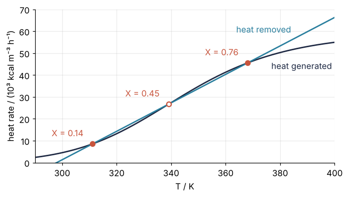
A reactor started cold settles at a conversion of 0.14, one started hot at 0.76, and the middle crossing divides them.

Pitfalls

success is True, and the answer is nonsense. Start from an impossible temperature:

r = root(residual, (0.5, -100.0))
print(r.success, r.message, r.x, r.fun)

True The solution converged. [   1.         -195.46968606] [-2.30942877e+10 -1.37641954e+14]

root reports convergence at X = 1 and −195.5 K, with an energy residual of −1.4e14 kcal/(m³ h). hybr stops when its steps become small compared with x, not when the residual is small. Never accept a result without the scaled-residual test of Step 5 and a look at whether the answer is physical, \(0 \le X \le 1\) and \(T > 0\).

Overflow warnings and a residual of inf. A start at −5 K is worse:

with warnings.catch_warnings(record=True) as caught:
    warnings.simplefilter("always")
    r = root(residual, (0.5, -5.0))
print(len(caught), "x", caught[0].message, "|", r.success, r.fun)

7 x overflow encountered in exp | False [inf inf]

Seven overflow warnings, a residual of inf, and success False. At \(T = -5\) K the Arrhenius factor is \(e^{+1192}\), which no float can hold. The cause is a start where the model means nothing. Draw starts from the physical box, as the grid does, or bound the unknowns (see Variations).

Rows on very different scales. The energy row is 10⁴ times the mass row, and at the cold state \(T\) is 2,000 times \(X\). hybr hardly notices, because MINPACK rescales the unknowns itself through its diag option, one factor per unknown, chosen by default from the Jacobian. Other methods do notice. method="krylov" never builds the Jacobian; it estimates the effect of \(J\) on a step from extra residual calls.

for f in [residual, scaled_residual]:
    r = root(f, (0.0, 300.0), method="krylov")
    print(f"{f.__name__:15s} success = {r.success!s:5s}  iterations = {r.nit:3d}  T = {r.x[1]:.2f} K")

residual        success = False  iterations = 300  T = 311.79 K
scaled_residual success = True   iterations =   4  T = 311.17 K

On the raw residual it gives up after 300 iterations; on the scaled one it converges in 4, with \(T\) left unscaled. Make every row order one before you choose a method, and judge the residual in those units.

Variations

• The other MINPACK interfaces. fsolve is the older interface to the same hybr code, common in older scripts, and new code should call root. With fprime=jacobian and full_output=True it takes the same 9 calls to the same answer and reports success as the integer ier, 1; without full_output it returns a bare array. method="lm", Levenberg-Marquardt, treats the system as a least-squares problem and needs 18 calls from the feed state; through scipy.optimize.least_squares it also takes more equations than unknowns, as in Earthquake location from three seismograms.
• Keeping the unknowns physical. least_squares(scaled_residual, x0, jac=..., bounds=([0, 250], [1, 500])) never leaves \(0 \le X \le 1\) and finds the cold state in 7 evaluations. The start must lie inside the bounds.
• A sweep in the jacket temperature. Loop \(T_j\) from 290 K upward and start each solve from the previous solution. The cold state is lost at 306 K: that is ignition, where the cold branch ends. Following a branch around such a turn is called continuation.
• Large systems. A tubular reactor discretized along its length has thousands of unknowns. method="krylov" or scipy.optimize.newton_krylov never forms the Jacobian, so the scaling of the third pitfall is the first thing to get right.

Cheat sheet

res = root(f, x0, jac=J)                        # f(x) returns an array as long as x, J(x) returns df_i/dx_j
approx_fprime(x, f)                             # finite-difference Jacobian, to check J
res.x, res.fun, res.success, res.message, res.nfev
scale = np.array([s1, s2])                      # each row's largest term at ordinary conditions
def ok(r): return r.success and np.all(np.abs(r.fun / scale) < 1e-8)   # success alone is not enough
starts = [(X0, T0) for X0 in X0s for T0 in T0s]                         # a grid over the physical box
sols = np.array(sorted((r.x for x0 in starts if ok(r := root(f, x0, jac=J))), key=lambda u: u[1]))
states = np.split(sols, np.nonzero(np.diff(sols[:, 1]) > 0.1)[0] + 1)   # new state where T jumps > 0.1 K
root(f, x0, method="lm")                        # least squares; "krylov" for very large systems
x, info, ier, msg = fsolve(f, x0, fprime=J, full_output=True)  # ier == 1 means converged

Further reading

• scipy.optimize.root reference, with the list of methods and their options, and the root finding section of the SciPy optimization tutorial.
• H. Scott Fogler, Elements of Chemical Reaction Engineering, section 12.5 of the 5th and 6th editions, on multiple steady states, for heat generated and heat removed.
• B. Wayne Bequette, Process Dynamics: Modeling, Analysis, and Simulation (Prentice Hall, 1998), Module 9, the source of the parameters and of the three solutions.
• C. van Heerden, "Autothermic Processes. Properties and Reactor Design", Industrial & Engineering Chemistry 45(6), 1242-1247 (1953), after whom the picture of heat generated against heat removed is named.
• Related tutorials on this site: Root finding with scipy.optimize: Halley's comet from Kepler's equation, Minimization with scipy.optimize.minimize: the shape of a seven-atom cluster for the same result object and restarts from many starts, Derive a Jacobian with SymPy and pass it to solve_ivp with lambdify to derive the Jacobian of Step 4 symbolically, and Earthquake location from three seismograms: circles, S minus P, and the misfit for least_squares on an overdetermined system. Planned: the same reactor in Julia with NonlinearSolve.jl.
• Download the notebook. It was executed with the library versions in the header.