Polynomial roots are eigenvalues: why Wilkinson's polynomial loses its roots (Python)

The question

Wilkinson's polynomial W(x) = (x − 1)(x − 2)⋯(x − 20) has the integers 1 to 20 as its roots, by construction. Multiply it out into its 21 coefficients, from x²⁰ down to the constant, and hand them to np.roots, the function most people reach for to find the roots of a polynomial in Python:

Show code

import mpmath
import numpy as np
import matplotlib.pyplot as plt
from math import prod
from numpy.polynomial import Chebyshev, Polynomial

plt.rcParams.update({
    "figure.figsize": (8, 3.2), "figure.dpi": 110,
    "axes.spines.top": False, "axes.spines.right": False,
    "axes.grid": True, "grid.alpha": 0.25,
    "font.size": 11, "lines.linewidth": 1.8,
})
INK, ACCENT, SECOND, MUTED = "#1f2a44", "#c8553d", "#2a7f9e", "#8a8f98"

mpmath.mp.dps = 60                             # 60 digits for every reference root
eps = np.finfo(float).eps
j = np.arange(1, 21)                           # the exact roots
powers = np.arange(20, -1, -1)                 # x²⁰ ... x⁰, highest first, as np.roots wants

# the exact coefficients of (x - 1)(x - 2)...(x - 20), in Python integers
exact = [1]
for k in range(1, 21):
    exact = [a - k * b for a, b in zip(exact + [0], [0] + exact)]
coef = np.array(exact, dtype=float)


def W(x):
    """Wilkinson's polynomial in factored form, which cancels nothing."""
    return np.prod([x - k for k in range(1, 21)], axis=0)


def mp_roots(c):
    """Roots of a polynomial with mpmath coefficients, sorted by real, then imaginary part."""
    r = mpmath.polyroots(c, maxsteps=500, extraprec=500)
    return np.array(sorted((complex(z) for z in r), key=lambda z: (round(z.real, 9), z.imag)))


inexact = [int(p) for p, a, c in zip(powers, exact, coef) if int(c) != a]
print(f"largest coefficient {max(map(abs, exact)):.3g}, constant 20! = {exact[-1]:.3g}, 2⁵³ = {2.0**53:.2g}")
print(f"rounded in float64: the coefficients of x^{min(inexact)} to x^{max(inexact)}")

r = np.roots(coef)
print(f"largest imaginary part {np.abs(r.imag).max()}\n")
r = np.sort(r.real)
print(" j    np.roots        error      j    np.roots        error")
for a in range(10):
    left, right = a, a + 10
    print(f"{j[left]:2d}  {r[left]:12.8f}  {abs(r[left] - j[left]):9.1e}     "
          f"{j[right]:2d}  {r[right]:12.8f}  {abs(r[right] - j[right]):9.1e}")

largest coefficient 1.38e+19, constant 20! = 2.43e+18, 2⁵³ = 9e+15
rounded in float64: the coefficients of x^3 to x^7
largest imaginary part 0.0

 j    np.roots        error      j    np.roots        error
 1    1.00000000    3.0e-13     11   11.02502293    2.5e-02
 2    2.00000000    2.8e-11     12   11.95328325    4.7e-02
 3    3.00000000    4.1e-10     13   13.07431403    7.4e-02
 4    3.99999998    1.6e-08     14   13.91475559    8.5e-02
 5    5.00000067    6.7e-07     15   15.07549380    7.5e-02
 6    5.99998925    1.1e-05     16   15.94628672    5.4e-02
 7    7.00010200    1.0e-04     17   17.02542715    2.5e-02
 8    7.99935583    6.4e-04     18   17.99092135    9.1e-03
 9    9.00291529    2.9e-03     19   19.00190982    1.9e-03
10    9.99041304    9.6e-03     20   19.99980929    1.9e-04

The root at 1 is off by 3 × 10⁻¹³, the one at 14 comes back as 13.9148. Part of that is the input. The coefficients reach 1.38 × 10¹⁹, the one of x², and an integer beyond 2⁵³ = 9.0 × 10¹⁵ is a float only if it has enough factors of two (Floating-point numbers). Five of them, those of x³ to x⁷, do not, and were rounded before the solver saw them.

Then there is the experiment Wilkinson made famous. He changed the coefficient of x¹⁹, which is −210, by 2⁻²³ ≈ 1.19 × 10⁻⁷. That is the seventh decimal place, or the tenth significant digit: a relative change of 5.7 × 10⁻¹⁰.

Show code

h_w = 2.0**-23
coef_h = coef.copy()
coef_h[1] -= h_w                               # -210 - 2⁻²³ is exact in float64
exact_h = [mpmath.mpf(a) for a in exact]
exact_h[1] -= mpmath.mpf(h_w)
ref_h = mp_roots(exact_h)
num_h = np.array(sorted(np.roots(coef_h), key=lambda z: (round(z.real, 9), z.imag)))

print(f"relative change of the x¹⁹ coefficient: {h_w / 210:.2g}\n")
print("roots of the changed polynomial, 60-digit mpmath:")
for z in ref_h[ref_h.imag >= 0]:
    print(f"   {z.real:11.6f}" + (f" ± {z.imag:.6f}i" if z.imag > 0 else ""))
print(f"\nnp.roots differs from them by at most {np.abs(num_h - ref_h).max():.1e}")

fig, ax = plt.subplots(figsize=(8, 3.2))
ax.axhline(0, color=MUTED, lw=1)
ax.plot(j, np.zeros(20), "o", mfc="none", mec=INK, ms=7, mew=1.2)
ax.plot(ref_h.real, ref_h.imag, "o", color=ACCENT, ms=5)
widest = ref_h[np.argmax(ref_h.imag)]
ax.annotate(f"{widest.real:.2f} ± {widest.imag:.2f}i", (widest.real, widest.imag),
            xytext=(0, 7), textcoords="offset points", ha="center", va="bottom", color=ACCENT)
ax.text(0.5, -1.0, "roots of W: 1, 2, …, 20", color=INK)
ax.text(0.5, -2.4, "after the change of 2⁻²³", color=ACCENT)
ax.set(xlabel="Re x", ylabel="Im x", xlim=(0, 22), ylim=(-3.5, 3.9), xticks=range(0, 23, 2))
plt.show()

relative change of the x¹⁹ coefficient: 5.7e-10

roots of the changed polynomial, 60-digit mpmath:
      1.000000
      2.000000
      3.000000
      4.000000
      5.000000
      6.000007
      6.999697
      8.007268
      8.917250
     10.095266 ± 0.643501i
     11.793634 ± 1.652330i
     13.992358 ± 2.518830i
     16.730737 ± 2.812625i
     19.502439 ± 1.940330i
     20.846908

np.roots differs from them by at most 1.4e-03

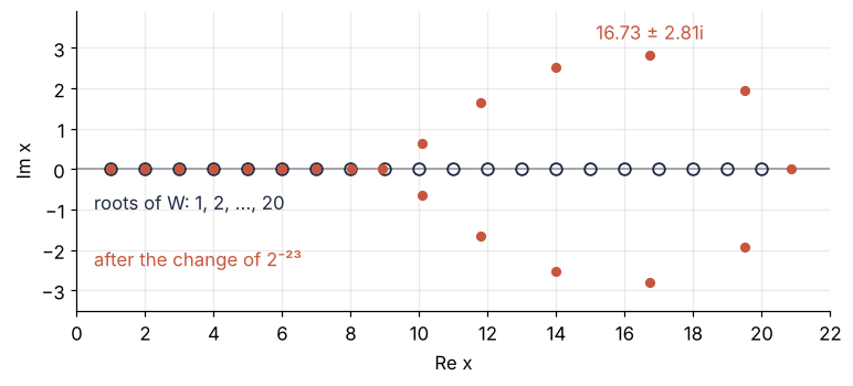
The complex plane, Re x from 0 to 22. Open circles: the roots 1 to 20 of W. Red dots: the roots after the coefficient of x¹⁹ changes by 2⁻²³. Up to 9 they sit on the circles; ten roots form five complex pairs, the widest at 16.73 ± 2.81i.

Half the roots leave the real axis. From 10 on they have paired up into five complex pairs, the widest at 16.7307 ± 2.8126i, and the real roots on either side of the pairs have moved to 8.9173 and 20.8469. np.roots agrees with a 60-digit computation by mpmath to 1.4 × 10⁻³: the changed polynomial really has these roots.

The obvious suspect is still the solver, which was already off by 0.085 near 14 before anyone touched a coefficient. The other suspect is the polynomial, or rather the way it is written down. Is np.roots broken, or is it giving honest answers to a question whose answer moves with the tenth digit of the data? The test comes at the end: 200 copies of W with every coefficient changed at random by one part in 10¹⁰, and for each root a number, computed before any copy is solved, that predicts how far it will scatter.

The idea: a matrix whose eigenvalues are the roots

np.roots does not hunt for the roots one at a time. It builds a matrix whose eigenvalues are the roots and hands that to an eigenvalue solver (Eigenvalues with numpy.linalg), which returns all of them at once. For a monic polynomial p(x) = xⁿ + aₙ₋₁xⁿ⁻¹ + ⋯ + a₀, put −aₙ₋₁, …, −a₀ in the first row of an n × n matrix C, ones just below the diagonal, and zeros everywhere else.

Multiply C by the vector v = (rⁿ⁻¹, …, r, 1). Each row below the first copies the entry of v one place up, which is r times the entry in its own place. The first row gives −aₙ₋₁rⁿ⁻¹ − ⋯ − a₀, which is rⁿ − p(r). So Cv = rv exactly when p(r) = 0: every root of p is an eigenvalue of C. For n distinct roots these are all n eigenvalues, so the characteristic polynomial det(xI − C) is p itself, and that identity holds for repeated roots too. This C is called the companion matrix of p. Here it is for (x − 1)(x − 2)(x − 3) = x³ − 6x² + 11x − 6:

Show code

def companion(c):
    """Companion matrix of a monic polynomial, coefficients highest first."""
    n = len(c) - 1
    C = np.zeros((n, n))
    C[0] = -np.asarray(c[1:], dtype=float)
    C[1:, :-1] = np.eye(n - 1)
    return C


C3 = companion([1, -6, 11, -6])
print(C3)
print(f"eigenvalues: {np.sort(np.linalg.eigvals(C3).real)}")
print(f"C · (4, 2, 1) = {C3 @ [4, 2, 1]}")

[[  6. -11.   6.]
 [  1.   0.   0.]
 [  0.   1.   0.]]
eigenvalues: [1. 2. 3.]
C · (4, 2, 1) = [8. 4. 2.]

The eigenvalues are 1, 2, and 3, and C times (4, 2, 1), the vector for r = 2, is (8, 4, 2). The companion matrix of W is 20 × 20, with 210 at the start of its first row and −20! at the end. Build it by hand and compare its eigenvalues with what np.roots returned:

Show code

C = companion(coef)
diff = np.abs(np.linalg.eigvals(C) - np.roots(coef)).max()
print(f"largest |eigvals(C) - np.roots(coef)| = {diff}")

largest |eigvals(C) - np.roots(coef)| = 0.0

The difference is 0.0, to the last bit, because building this matrix and calling the eigenvalue solver is all np.roots does. That moves the question. Like the LU solve of The condition number, the eigenvalue solver is backward stable: its answers are the exact eigenvalues of a matrix changed by a few ε. So where do an error of 0.085 and an imaginary part of 2.8 come from?

Why a change of 10⁻⁷ moves a root by 3

Wilkinson's change turns W(x) into W(x) − h x¹⁹ with h = 2⁻²³. Divide the equation W(x) − h x¹⁹ = 0 by x¹⁹ and it becomes a picture: the roots are the points where the curve W(x)/x¹⁹ meets the horizontal line at height h.

Since h is positive, the line can only cross where W(x)/x¹⁹ is positive. For x < 0 the quotient is negative, W being positive and x¹⁹ negative. For x > 0 the sign of W flips at every integer, and W is positive on (0, 1), (2, 3), (4, 5), and so on up to (18, 19), and beyond 20. The two outer intervals give one crossing each: on (0, 1) the curve falls from infinity to zero, beyond 20 it rises from zero without bound. On each of the nine intervals from (2, 3) to (18, 19) the curve rises from zero to a hump and falls back, two crossings as long as the line stays below the top. That makes twenty. The tops of the humps decide everything:

Show code

humps = {}
for a in range(2, 19, 2):
    x = a + np.linspace(0, 1, 20001)
    humps[a] = (W(x) / x**19).max()
    print(f"hump on ({a:2d}, {a + 1:2d}):  top of W(x)/x¹⁹ = {humps[a]:.3g}")

heights = [1e-10, 3e-10, h_w]
real_counts = []
for h in heights:
    c = [mpmath.mpf(a) for a in exact]
    c[1] -= mpmath.mpf(h)
    real_counts.append(int(np.sum(np.abs(mp_roots(c).imag) < 1e-20)))
print()
for h, n in zip(heights, real_counts):
    print(f"h = {h:8.3g}:  {n} real roots, humps below the line: "
          f"{[f'({a}, {a + 1})' for a in humps if humps[a] < h]}")

hump on ( 2,  3):  top of W(x)/x¹⁹ = 3.77e+08
hump on ( 4,  5):  top of W(x)/x¹⁹ = 26.1
hump on ( 6,  7):  top of W(x)/x¹⁹ = 0.00143
hump on ( 8,  9):  top of W(x)/x¹⁹ = 1.87e-06
hump on (10, 11):  top of W(x)/x¹⁹ = 1.9e-08
hump on (12, 13):  top of W(x)/x¹⁹ = 9.39e-10
hump on (14, 15):  top of W(x)/x¹⁹ = 1.84e-10
hump on (16, 17):  top of W(x)/x¹⁹ = 1.42e-10
hump on (18, 19):  top of W(x)/x¹⁹ = 5.71e-10

h =    1e-10:  20 real roots, humps below the line: []
h =    3e-10:  16 real roots, humps below the line: ['(14, 15)', '(16, 17)']
h = 1.19e-07:  10 real roots, humps below the line: ['(10, 11)', '(12, 13)', '(14, 15)', '(16, 17)', '(18, 19)']

The humps on the left are enormous, 3.77 × 10⁸ on (2, 3), and they shrink fast: 1.87 × 10⁻⁶ on (8, 9), 1.90 × 10⁻⁸ on (10, 11), down to 1.42 × 10⁻¹⁰ on (16, 17). Wilkinson's h = 1.19 × 10⁻⁷ is higher than five of them, every hump from (10, 11) on. When the line rises past the top of a hump, its two crossings move toward the top, meet there, and the pair leaves the real axis as complex conjugates. Five humps, five pairs.

Show code

# W > 0 on (8, 9), ..., (18, 19) and beyond 20; points crowd toward the zeros of W
ends = np.sin(np.linspace(0, np.pi / 2, 400)) ** 2
segments = [a + ends for a in range(8, 20, 2)] + [20 + 2 * ends]
labels = ["h = 10⁻¹⁰", "h = 3 × 10⁻¹⁰", "h = 2⁻²³"]

fig, axes = plt.subplots(3, 1, figsize=(8, 6.3), sharex=True)
for ax, h, label, n in zip(axes, heights, labels, real_counts):
    for x in segments:
        ax.semilogy(x, W(x) / x**19, color=INK)
    ax.axhline(h, color=SECOND, lw=1.2)
    c = [mpmath.mpf(a) for a in exact]
    c[1] -= mpmath.mpf(h)
    rh = mp_roots(c)
    cross = rh[(np.abs(rh.imag) < 1e-20) & (rh.real > 7)].real
    ax.plot(cross, np.full(cross.size, h), "o", color=ACCENT, ms=6)
    ax.text(0.36, 0.95, f"{label}:  {n} real roots", transform=ax.transAxes, va="top")
    ax.set(ylabel="W(x) / x¹⁹", ylim=(1e-11, 1e-5))
axes[-1].set(xlabel="x", xlim=(7, 22))
plt.show()

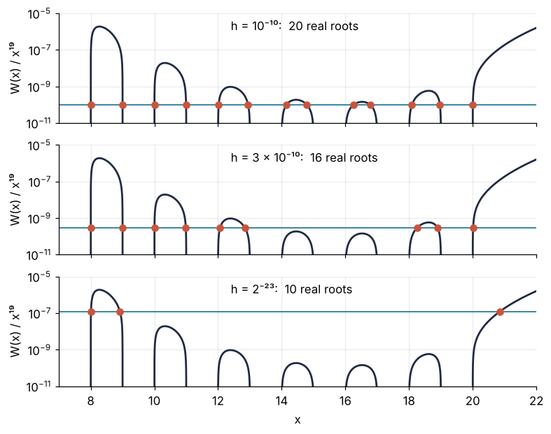
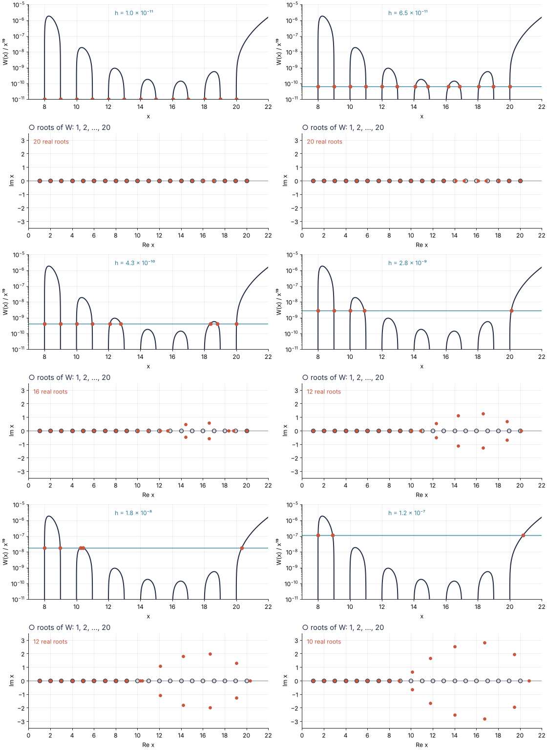
Three stacked panels of W(x)/x¹⁹ on a log axis from 10⁻¹¹ to 10⁻⁵, for x from 7 to 22, drawn where W is positive. A blue line at h = 10⁻¹⁰, 3 × 10⁻¹⁰, and 2⁻²³, red dots at its crossings with the curve: 20, 16, and 10 real roots.

At h = 10⁻¹⁰ the line passes under every hump and all 20 roots are real. At 3 × 10⁻¹⁰ it clears the two lowest, on (14, 15) and (16, 17), and 16 are left. At 2⁻²³ only 10 are. Watch the line rise continuously from 10⁻¹¹ to 2⁻²³, with the roots in the complex plane below:

Top: W(x)/x¹⁹ where W is positive, on a log axis, and a blue line at height h rising from 10⁻¹¹ to 2⁻²³. Bottom: the 20 roots of W(x) − h x¹⁹ in the complex plane. Each time the line passes the top of a hump, its two crossings meet and the pair leaves the real axis.

Show code

"""Root collision: the roots of W(x) - h x^19 as the line at height h rises.

W(x) = (x - 1)(x - 2)...(x - 20) is Wilkinson's polynomial. The roots of W(x) - h x^19
are the crossings of the curve W(x)/x^19 with the horizontal line at height h. When the
line passes the top of a hump, two real roots meet and leave the real axis as a pair.
Renders ../../assets/root-collision.gif. Run it from any directory:

    python scene.py
"""
from pathlib import Path

import mpmath
import numpy as np
import matplotlib.pyplot as plt
from matplotlib.animation import FuncAnimation, PillowWriter
from PIL import Image

OUT = Path(__file__).resolve().parents[2] / "assets" / "root-collision.gif"
INK, ACCENT, SECOND, MUTED = "#1f2a44", "#c8553d", "#2a7f9e", "#8a8f98"
plt.rcParams.update({"axes.spines.top": False, "axes.spines.right": False,
                     "axes.grid": True, "grid.alpha": 0.25, "font.size": 11})
mpmath.mp.dps = 60

# ---- data: the exact integer coefficients of W, highest power first
exact = [1]
for k in range(1, 21):
    exact = [a - k * b for a, b in zip(exact + [0], [0] + exact)]


def W(x):
    return np.prod([x - k for k in range(1, 21)], axis=0)


def roots_at(h):
    """Roots of W(x) - h x^19, from mpmath at 60 digits: np.roots is not accurate enough here."""
    c = [mpmath.mpf(a) for a in exact]
    c[1] -= mpmath.mpf(h)
    return np.array([complex(z) for z in mpmath.polyroots(c, maxsteps=500, extraprec=500)])


h_sweep = np.geomspace(1e-11, 2.0**-23, 96)
frames = np.concatenate([h_sweep, np.full(14, h_sweep[-1])])      # hold the last frame a second
roots = {h: roots_at(h) for h in h_sweep}                         # about 40 s, once

# W > 0 on (8, 9), (10, 11), ..., (18, 19) and beyond 20; points crowd toward the zeros
# so that the curve reaches the bottom of the log axis
ends = np.sin(np.linspace(0, np.pi / 2, 400)) ** 2
segments = [a + ends for a in range(8, 20, 2)] + [20 + 2 * ends]

# ---- figure, drawn once
fig, (ax1, ax2) = plt.subplots(2, 1, figsize=(7, 6.4), dpi=80, layout="constrained")
for x in segments:
    ax1.semilogy(x, W(x) / x**19, color=INK, lw=1.8)
line = ax1.axhline(1e-11, color=SECOND, lw=1.2)
(crossings,) = ax1.plot([], [], "o", color=ACCENT, ms=6)
h_text = ax1.text(0.36, 0.95, "", transform=ax1.transAxes, va="top", color=SECOND)
ax1.set(xlabel="x", ylabel="W(x) / x¹⁹", xlim=(7, 22), ylim=(1e-11, 1e-5))

ax2.axhline(0, color=MUTED, lw=1)
ax2.plot(np.arange(1, 21), np.zeros(20), "o", mfc="none", mec=INK, ms=7, mew=1.2)
(dots,) = ax2.plot([], [], "o", color=ACCENT, ms=5)
count_text = ax2.text(0.02, 0.95, "", transform=ax2.transAxes, va="top", color=ACCENT)
ax2.set(xlabel="Re x", ylabel="Im x", xlim=(0, 22), ylim=(-3.5, 3.5), xticks=range(0, 23, 2))
ax2.set_title("○ roots of W: 1, 2, …, 20", loc="left", color=INK)


def sci(h):
    """h as 5.6 × 10⁻⁹, with a superscript exponent."""
    e = int(np.floor(np.log10(h)))
    return f"{h / 10.0**e:.1f} × 10" + str(e).translate(str.maketrans("-0123456789", "⁻⁰¹²³⁴⁵⁶⁷⁸⁹"))


# ---- one frame: a function of h alone
def update(h):
    r = roots[h]
    real = r[np.abs(r.imag) < 1e-20].real
    line.set_ydata([h, h])
    shown = real[real > 7]
    crossings.set_data(shown, np.full(shown.size, h))
    h_text.set_text(f"h = {sci(h)}")
    dots.set_data(r.real, r.imag)
    count_text.set_text(f"{real.size} real roots")


# ---- render, and read back what was written
OUT.parent.mkdir(exist_ok=True)
FuncAnimation(fig, update, frames=frames).save(OUT, writer=PillowWriter(fps=12))
plt.close(fig)
with Image.open(OUT) as im:
    seconds = 0
    for i in range(im.n_frames):                                  # Pillow merges the held frames
        im.seek(i)
        seconds += im.info["duration"] / 1000
    print(f"{OUT.name}: {im.width} x {im.height} px, {im.n_frames} frames, "
          f"{seconds:.1f} s, {OUT.stat().st_size / 1024:,.0f} kB")

The pair from (16, 17) leaves first, at h = 1.42 × 10⁻¹⁰, and the one from (10, 11) last, at 1.90 × 10⁻⁸. Once off the axis, a pair keeps moving as h grows, which is how one of them got as far as 16.73 ± 2.81i.

Why so small an h matters is a question of sizes. At x = 16 the added term is h x¹⁹ = 2⁻²³ · 2⁷⁶ = 2⁵³ = 9.0 × 10¹⁵, while W itself between 15 and 16 never exceeds 5.9 × 10¹². W is that small because it is a sum of 21 terms aᵢxⁱ of up to 10²⁷ that cancel almost completely:

Show code

xm = mpmath.mpf("15.5")
terms = [abs(a) * xm**int(p) for a, p in zip(exact, powers)]
x = np.linspace(15, 16, 10001)
print(f"h x¹⁹ at x = 16:            {h_w * 16.0**19:.3g}")
print(f"largest |W(x)| on [15, 16]: {np.abs(W(x)).max():.3g}")
print(f"at x = 15.5: largest term {float(max(terms)):.3g}, |W| = {abs(W(15.5)):.3g}, "
      f"sum of |terms| / |W| = {float(sum(terms)) / abs(W(15.5)):.2g}")
dW16 = prod(16 - k for k in range(1, 21) if k != 16)
print(f"first-order move of the root 16 for h = 2⁻²³: h·16¹⁹/|W'(16)| = {h_w * 16.0**19 / abs(dW16):.0f}")

h x¹⁹ at x = 16:            9.01e+15
largest |W(x)| on [15, 16]: 5.93e+12
at x = 15.5: largest term 2.25e+27, |W| = 5.58e+12, sum of |terms| / |W| = 2.1e+15
first-order move of the root 16 for h = 2⁻²³: h·16¹⁹/|W'(16)| = 287

At x = 15.5 the absolute values of the terms add up to 2.1 × 10¹⁵ times W, so a change in the tenth digit of one coefficient is a change in the first digit of what is left after the cancellation. The first-order formula of the next section, h · 16¹⁹/|W′(16)| with W′(16) = 15! · 4!, would move the root at 16 by about 290. The roots do not move a little, they collide.

Formalization

For the companion matrix C of a monic polynomial p,

\[\det(xI - C) = p(x),\]

which is what the eigenvector above showed.

Change each coefficient aᵢ by δaᵢ and write the change as a polynomial, δp(x) = Σ δaᵢ xⁱ. A simple root r moves to r + δr with p(r + δr) + δp(r + δr) = 0, and to first order, since p(r) = 0, that is p′(r) δr + δp(r) = 0:

\[\delta r \approx -\frac{\delta p(r)}{p'(r)}.\]

If every coefficient changes by at most a relative η, |δaᵢ| ≤ η|aᵢ|, then |δp(rⱼ)| ≤ η Σ|aᵢ||rⱼ|ⁱ, and the root rⱼ moves by at most a relative κⱼ η, with

\[\kappa_j = \frac{\sum_i |a_i|\,|r_j|^i}{|r_j|\,|p'(r_j)|}.\]

The numerator is the size of the terms that cancel at the root, the denominator how steeply p crosses zero there. The absolute move is κⱼ η |rⱼ|. The table sets κⱼ ε j beside the errors of np.roots and adds κ̂ⱼ, computed from the float coefficients at the computed roots.

Show code

def kappa_monomial(c, x):
    """Relative condition number of the root x of the polynomial c (highest first)."""
    c = np.asarray(c, dtype=float)
    pw = np.arange(len(c) - 1, -1, -1)
    return np.sum(np.abs(c) * np.abs(x) ** pw) / (np.abs(x) * np.abs(np.polyval(np.polyder(c), x)))


dW = np.array([abs(prod(int(jj) - k for k in range(1, 21) if k != jj)) for jj in j], dtype=float)
kappa = np.array([np.sum(np.abs(coef) * float(jj) ** powers) for jj in j]) / (j * dW)
kappa_hat = np.array([kappa_monomial(coef, x) for x in r])
err = np.abs(r - j)
ratio = err / (kappa * eps * j)
shift = np.log10(kappa_hat) - np.log10(kappa)

print(" j      κ_j    error   κ_j·ε·j   error / (κ_j·ε·j)   log10 κ̂_j − log10 κ_j")
for i in range(20):
    print(f"{j[i]:2d}  {kappa[i]:7.2g}  {err[i]:7.2g}  {kappa[i] * eps * j[i]:8.2g}"
          f"  {ratio[i]:12.2f}  {shift[i]:+18.3f}")
print(f"\nerror / (κ_j·ε·j) from {ratio.min():.2f} to {ratio.max():.2f}; "
      f"κ at the computed roots within {np.abs(shift).max():.2f} in log10")

 j      κ_j    error   κ_j·ε·j   error / (κ_j·ε·j)   log10 κ̂_j − log10 κ_j
 1  4.2e+02    3e-13   9.3e-14          3.23              -0.000
 2  4.4e+04  2.8e-11   1.9e-11          1.45              +0.000
 3    2e+06  4.1e-10   1.3e-09          0.30              -0.000
 4  5.1e+07  1.6e-08   4.6e-08          0.36              -0.000
 5  8.2e+08  6.7e-07   9.1e-07          0.73              +0.000
 6  8.9e+09  1.1e-05   1.2e-05          0.90              -0.000
 7  6.9e+10   0.0001   0.00011          0.95              +0.000
 8  3.9e+11  0.00064    0.0007          0.93              -0.001
 9  1.7e+12   0.0029    0.0034          0.87              +0.002
10  5.6e+12   0.0096     0.012          0.78              -0.005
11  1.4e+13    0.025     0.035          0.72              +0.009
12  2.8e+13    0.047     0.076          0.62              +0.002
13  4.4e+13    0.074      0.13          0.58              +0.005
14  5.4e+13    0.085      0.17          0.51              +0.042
15    5e+13    0.075      0.17          0.45              -0.027
16  3.5e+13    0.054      0.13          0.43              +0.046
17  1.8e+13    0.025     0.068          0.37              -0.025
18  6.4e+12   0.0091     0.025          0.36              +0.013
19  1.4e+12   0.0019    0.0058          0.33              -0.003
20  1.4e+11  0.00019   0.00061          0.31              +0.001

error / (κ_j·ε·j) from 0.30 to 3.23; κ at the computed roots within 0.05 in log10

κⱼ runs from 420 at x = 1 to 5.4 × 10¹³ at x = 14, and the errors lie between 0.30 and 3.2 times κⱼ ε j.

Digits lost, log₁₀ κⱼ. As in the prerequisite, about 16 − log₁₀ κⱼ digits survive. At x = 14, κ = 5.4 × 10¹³ leaves two, and 13.9148 is what two digits look like; at x = 1, κ = 420 leaves 13. The rule works without the exact roots: compute κⱼ from your coefficients at the roots np.roots returned. For W that estimate, the table's last column, is within 0.05 of the exact log₁₀ κⱼ, because a root wrong in its third digit still gives κ the right order of magnitude.

What the solver adds. The eigenvalue solver returns the exact eigenvalues of a nearby matrix C + E, with E a few ε relative to the size of C: the exact roots of det(xI − C − E), a polynomial whose coefficients differ from p's by combinations of the entries of E. But C holds entries up to 1.38 × 10¹⁹, and ε times that is 3,065, enough to change the coefficient of x¹⁹, −210, by thousands. κⱼ needs each coefficient to move by a few ε of its own size. The solver first rescales rows and columns by powers of two, called balancing. Whether that is enough is measured here: the computed roots, multiplied out in 60 digits, against your coefficients.

Show code

back = [mpmath.mpc(1)]
for z in np.roots(coef):                       # multiply out the computed roots, 60 digits
    z = mpmath.mpc(z.real, z.imag)
    back = [a - z * b for a, b in zip(back + [0], [0] + back)]
rel = np.array([float(abs(b - mpmath.mpf(c)) / abs(c)) for b, c in zip(back, coef)]) / eps
print(f"largest entry of C {np.abs(coef).max():.3g}, times ε: {eps * np.abs(coef).max():.0f}")
print(f"backward error per coefficient: largest {rel.max():.1f} ε (x^{powers[rel.argmax()]}), "
      f"median {np.median(rel):.1f} ε, leading coefficient {rel[0]:.0f} ε")

rounded = mp_roots([mpmath.mpf(c) for c in coef])   # exact roots of the rounded coefficients
dev = np.abs(rounded - j)
print(f"rounding alone: largest move {dev.max():.2g} at x = {j[dev.argmax()]}, {dev[13]:.2g} at x = 14")

largest entry of C 1.38e+19, times ε: 3065
backward error per coefficient: largest 16.8 ε (x^3), median 3.4 ε, leading coefficient 0 ε
rounding alone: largest move 0.00062 at x = 13, 0.00055 at x = 14

Every coefficient comes back within 17ε of its own size, the median within 3.4ε, so balancing is enough: η is a few ε, which is why the ratios in the table stay within a factor of about 3 of one. Rounding the coefficients to floats accounts for little: their exact roots are off by at most 6.2 × 10⁻⁴, at x = 13. The rest of the 0.085 at x = 14 is the solver's few ε, amplified by κⱼ. np.roots is not broken: it answers exactly for coefficients within 17ε of yours.

The basis decides. κⱼ depends on the coefficients, and they depend on the basis. Map [0, 21] onto [−1, 1] with s = (2x − 21)/21 and write W = Σ cₖ Tₖ(s), with the Chebyshev polynomials Tₖ(cos θ) = cos kθ. No |Tₖ| exceeds 1 there, so the terms add up in size to at most Σ|cₖ|, for W 2.4 × 10¹⁸, its own largest value on [0, 21]. Chebyshev.interpolate at degree 20 samples W at 21 Chebyshev points, the cosines of 21 equally spaced angles mapped onto [0, 21]. Since 21 values fix a polynomial of degree 20, the interpolant is W itself, to a few ε per value. κⱼ is the same formula with |cₖ||Tₖ(s(rⱼ))| in place of |aᵢ||rⱼ|ⁱ:

Show code

cheb = Chebyshev.interpolate(W, 20, domain=[0, 21])


def kappa_chebyshev(p, x):
    """The same condition number, with the Chebyshev terms |c_k||T_k(s)| in the numerator."""
    s = (2 * x - 21) / 21
    T = np.polynomial.chebyshev.chebvander(s, 20)
    return np.sum(np.abs(p.coef) * np.abs(T)) / (abs(x) * abs(p.deriv()(x)))


kappa_cheb = np.array([kappa_chebyshev(cheb, float(jj)) for jj in j])
s = (2 * 15.5 - 21) / 21
cancel = np.sum(np.abs(cheb.coef * np.polynomial.chebyshev.chebvander(s, 20))) / abs(W(15.5))
print(f"Chebyshev κ_j from {kappa_cheb.min():.2g} to {kappa_cheb.max():.2g} (at x = {j[kappa_cheb.argmax()]}), "
      f"monomial up to {kappa.max():.2g}")
print(f"sum of |c_k| {np.abs(cheb.coef).sum():.3g}, largest |W| on [0, 21] {np.abs(W(np.linspace(0, 21, 210001))).max():.3g}")
print(f"at x = 15.5: sum of |Chebyshev terms| / |W| = {cancel:.2g}")

Chebyshev κ_j from 0.64 to 1.8e+05 (at x = 10), monomial up to 5.4e+13
sum of |c_k| 2.43e+18, largest |W| on [0, 21] 2.43e+18
at x = 15.5: sum of |Chebyshev terms| / |W| = 2.9e+05

Its maximum is 1.8 × 10⁵, at x = 10, eight orders of magnitude below the monomial 5.4 × 10¹³, because at x = 15.5 the Chebyshev terms cancel by a factor of only 2.9 × 10⁵. The basis helps only if the polynomial never passes through the expanded monomial coefficients: converting those carries their damage along. In factored form the roots are the data, and nothing is lost at all.

See it in code

Four routes to the roots of W, then the test from the beginning: 200 copies of W with every coefficient multiplied by 1 + 10⁻¹⁰ g, g standard normal, through np.roots, and the same changes on the Chebyshev coefficients.

Show code

routes = {
    "np.roots, float coefficients": np.roots(coef),
    "Polynomial(coef[::-1]).roots()": Polynomial(coef[::-1]).roots(),
    "converted to Chebyshev on [0, 21]": Polynomial(coef[::-1]).convert(kind=Chebyshev, domain=[0, 21]).roots(),
    "Chebyshev.interpolate of the product": cheb.roots(),
}
for name, roots in routes.items():
    worst = np.abs(np.sort_complex(roots) - j).max()      # a complex root counts with its imaginary part
    print(f"{name:37s} worst error {worst:8.2g}, largest |Im| {np.abs(roots.imag).max():.2g}")

eta = 1e-10
rng = np.random.default_rng(0)
g = rng.standard_normal((200, 21))
cloud = np.array([np.sort_complex(np.roots(coef * (1 + eta * gi))) for gi in g])
cheb_moves = np.array([np.abs(np.sort(Chebyshev(cheb.coef * (1 + eta * gi), domain=[0, 21]).roots()) - j).max()
                       for gi in g])
print()
for i in range(5):                             # the roots that stay near their integer
    move = np.abs(cloud[:, i] - j[i]).max()
    print(f"cloud at x = {j[i]}: largest move {move:7.2g}, κ·η·j = {kappa[i] * eta * j[i]:7.2g}, "
          f"largest |Im| {np.abs(cloud[:, i].imag).max():.2g}")
print(f"whole cloud: largest |Im| {np.abs(cloud.imag).max():.2g}")
print(f"same changes, Chebyshev coefficients: largest move {cheb_moves.max():.2g}, "
      f"largest κ·η·j {(kappa_cheb * eta * j).max():.2g}")

fig, ax = plt.subplots(figsize=(8, 3.6))
ax.axhline(0, color=MUTED, lw=1)
ax.plot(cloud.real.ravel(), cloud.imag.ravel(), "o", color=ACCENT, ms=2.5, alpha=0.4, mew=0)
ax.plot(j, np.zeros(20), "o", mfc="none", mec=INK, ms=7, mew=1.2)
for jj, k in zip(j, kappa):
    ax.text(jj, 6.4 if jj % 2 else 7.6, f"{np.log10(k):.1f}", ha="center", va="bottom", color=INK)
ax.text(23, 6.4, "log₁₀ κⱼ", ha="right", va="bottom", color=INK)
ax.set(xlabel="Re x", ylabel="Im x", xlim=(0, 23), ylim=(-6.5, 9), xticks=range(0, 23, 2))
plt.show()

np.roots, float coefficients          worst error    0.085, largest |Im| 0
Polynomial(coef[::-1]).roots()        worst error     0.56, largest |Im| 0.21
converted to Chebyshev on [0, 21]     worst error   0.0095, largest |Im| 0
Chebyshev.interpolate of the product  worst error  6.4e-10, largest |Im| 0

cloud at x = 1: largest move 6.1e-08, κ·η·j = 4.2e-08, largest |Im| 0
cloud at x = 2: largest move   1e-05, κ·η·j = 8.8e-06, largest |Im| 0
cloud at x = 3: largest move 0.00072, κ·η·j = 0.00061, largest |Im| 0
cloud at x = 4: largest move   0.026, κ·η·j =   0.021, largest |Im| 0
cloud at x = 5: largest move    0.49, κ·η·j =    0.41, largest |Im| 0.48
whole cloud: largest |Im| 5.5
same changes, Chebyshev coefficients: largest move 0.00021, largest κ·η·j 0.00018

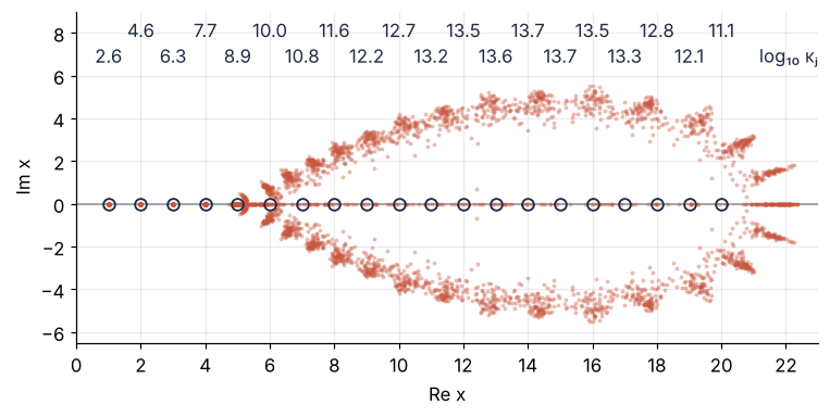
The complex plane, Re x from 0 to 23, with the roots of 200 copies of W whose coefficients changed by 10⁻¹⁰ at random. Up to 4 the roots stay on the circles; from 5 on they spread into a ring reaching 5.5 into the plane. A row labeled log₁₀ κⱼ above the integers runs from 2.6 at x = 1 to 13.7 at x = 14 and 15.

np.roots misses by 0.085. Polynomial.roots misses by 0.56 and turns the roots at 14 and 15 into the pair 14.52 ± 0.21i: Polynomial puts its coefficients in the last column of its companion matrix, which changes the backward error, not the conditioning. Converting the float coefficients to Chebyshev form gets 9.5 × 10⁻³, better than either, and seven orders of magnitude behind the interpolant of the factored product at 6.4 × 10⁻¹⁰. Chebyshev.roots is again an eigenvalue problem, of the colleague matrix, the companion matrix of the Chebyshev basis. Their last digits depend on the linear algebra library behind your NumPy.

The clouds follow the printed log₁₀ κⱼ. From x = 1 to 5 the largest move is within 1.5 times κ η j (6.1 × 10⁻⁸ against 4.2 × 10⁻⁸ at x = 1), and at x = 5, where κ η j = 0.41, the first roots leave the axis. Beyond, κ η j exceeds 1, first order says only that the root is lost, and the roots spread into a ring reaching 5.5 into the plane. On the Chebyshev coefficients they move no root by more than 2.1 × 10⁻⁴, against a largest κ η j of 1.8 × 10⁻⁴, and every root stays real.

Where it shows up

Wherever a model is a polynomial, κⱼ decides whether np.roots can be trusted with its roots. The cell computes the numbers quoted below.

Show code

import scipy.signal

# linear algebra: a symmetric matrix with eigenvalues 1 to 20
rng_q = np.random.default_rng(1)
Q, _ = np.linalg.qr(rng_q.standard_normal((20, 20)))
B = Q @ np.diag(j.astype(float)) @ Q.T
B = (B + B.T) / 2
via_poly = np.roots(np.poly(B))                # np.poly multiplies out the eigenvalues of B
print(f"eigvalsh error {np.abs(np.linalg.eigvalsh(B) - j).max():.2g}, "
      f"np.roots(np.poly(B)) error {np.abs(np.sort(via_poly.real) - j).max():.2g}")

# chemistry: van der Waals CO2 at 280 K and 50 bar, cubic in the molar volume V
R, a_vdw, b_vdw, T, p = 8.314462618, 0.3640, 4.267e-5, 280.0, 50e5
cubic = [p, -(p * b_vdw + R * T), a_vdw, -a_vdw * b_vdw]
V = np.sort(np.roots(cubic).real)
print(f"van der Waals V = {', '.join(f'{v * 1e3:.4f}' for v in V)} L/mol, "
      f"κ = {', '.join(f'{kappa_monomial(cubic, v):.2g}' for v in V)}")

# engineering: Butterworth low-pass poles from the denominator vs SciPy's designed poles
for N in [8, 16, 24]:
    _, a_ba = scipy.signal.butter(N, 0.1, output="ba")
    _, poles, _ = scipy.signal.butter(N, 0.1, output="zpk")
    z = np.roots(a_ba)
    miss = max(np.abs(poles - zi).min() for zi in z)
    print(f"Butterworth order {N:2d}: poles misplaced by {miss:.2g}, largest |z| {np.abs(z).max():.3f}")

# physics: two cold beams at ±v0, each with plasma frequency ωp; ω in units of ωp, K = k v0 / ωp
def two_stream(K):
    return [1, 0, -2 * (K**2 + 1), 0, K**4 - 2 * K**2]

K = np.linspace(0.01, 1.5, 14901)
growth = np.array([np.roots(two_stream(k)).imag.max() for k in K])
quartic_roots = np.roots(two_stream(np.sqrt(3) / 2))
print(f"two-stream: largest growth rate {growth.max():.4f} ωp at k v0 = {K[growth.argmax()]:.3f} ωp "
      f"(√3/2 = {np.sqrt(3) / 2:.3f}), κ = {max(kappa_monomial(two_stream(np.sqrt(3) / 2), w) for w in quartic_roots):.2f}")

eigvalsh error 1.1e-14, np.roots(np.poly(B)) error 0.066
van der Waals V = 0.0823, 0.1257, 0.3003 L/mol, κ = 17, 23, 8.6
Butterworth order  8: poles misplaced by 4.3e-10, largest |z| 0.941
Butterworth order 16: poles misplaced by 0.029, largest |z| 0.970
Butterworth order 24: poles misplaced by 0.4, largest |z| 1.191
two-stream: largest growth rate 0.5000 ωp at k v0 = 0.866 ωp (√3/2 = 0.866), κ = 0.94

Linear algebra: characteristic polynomials. A symmetric 20 × 20 matrix B = Q diag(1, …, 20) Qᵀ with a random orthogonal Q has its eigenvalues found by eigvalsh to 1.1 × 10⁻¹⁴, but np.roots(np.poly(B)), where np.poly multiplies those eigenvalues out into the characteristic polynomial, gets them back only to 0.066. Eigenvalue solvers never form the characteristic polynomial for this reason, and np.roots runs the same road in the opposite direction.
Chemistry: cubic equations of state. The van der Waals equation for CO₂ (a = 0.3640 Pa m⁶ mol⁻², b = 4.267 × 10⁻⁵ m³ mol⁻¹) at 280 K and 50 bar is a cubic in the molar volume with three real roots, 0.0823, 0.126, and 0.300 L/mol: the liquid, the unstable middle, and the gas. Their κⱼ are 17, 23, and 8.6, so np.roots keeps about 14 digits and is the right tool.
Engineering: filter design. The poles of a digital Butterworth low-pass filter are the roots of the denominator polynomial that scipy.signal.butter(N, 0.1, output="ba") returns, and they must lie inside the unit circle |z| < 1 for the filter to be stable; np.roots misplaces them by 4.3 × 10⁻¹⁰ at order 8 and 0.029 at order 16, and at order 24 puts one at radius 1.19, an unstable filter from a stable design. SciPy's output="sos" keeps the filter as a product of second-order factors, the factored form again (Filtering with scipy.signal).
Physics: plasma waves. Two cold electron beams streaming through each other at ±v₀, each with plasma frequency ωₚ, give a quartic dispersion relation in the frequency ω, and its complex roots are the two-stream instability, growing fastest, at ωₚ/2, when kv₀ = (√3/2)ωₚ. All four roots have κ = 0.94 there, so degree 4 is no danger.

Spacing is not the criterion, κⱼ is: Wilkinson's roots are a full unit apart. Compute it from your own coefficients at the roots you got, as above, and when 16 − log₁₀ κⱼ leaves fewer digits than you need, which happens at high degree with many real roots along an interval, keep the polynomial factored or build it in a basis fitted to that interval from its values, never from expanded coefficients.

The question

The idea: a matrix whose eigenvalues are the roots

Why a change of 10⁻⁷ moves a root by 3

Formalization

See it in code

Where it shows up

Further reading