Split-step Fourier for the nonlinear Schrödinger equation: solitons in a fiber (Python)

The problem: how far does a soliton travel unchanged in a fiber?

A 1 ps pulse of 1550 nm light enters a standard single-mode fiber. A weak pulse has doubled its rms width after 136 m; at 15.4 W peak power the same pulse keeps its shape for kilometers. That pulse is a soliton of the nonlinear Schrödinger equation, and split-step Fourier is the method that computes it. The 1 ps is \(T_0\) in \(\mathrm{sech}(T/T_0)\), not the full width at half maximum. The light is the carrier wave times an envelope \(A(z, T)\) that changes slowly compared with it, and \(|A|^2\) is the power in W.

Two effects compete. The fiber's dispersion is anomalous, \(\beta_2 \approx -20\) ps²/km: higher frequencies travel faster. Alone it spreads the pulse over the dispersion length \(L_D = T_0^2/|\beta_2|\) = 50 m and chirps it, so that its frequency changes from front to back. The Kerr effect makes the refractive index grow with intensity, turns the phase by one radian over the nonlinear length \(L_{NL} = 1/(\gamma P)\), with γ = 1.3 /(W km), and chirps the pulse the opposite way. At \(L_{NL} = L_D\) the two cancel. In Agrawal's form, losses neglected,

\[\frac{\partial A}{\partial z} = -\frac{i\beta_2}{2}\,\frac{\partial^2 A}{\partial T^2} + i\gamma\,|A|^2 A ,\]

with z the distance along the fiber and T the time in a frame that moves with the pulse. Dispersion alone is solved exactly in Fourier space, the Kerr term alone exactly in time, so the method alternates the two in short steps of z. After 1 km in 1000 steps of 1 m, how far is the computed soliton from the exact one?

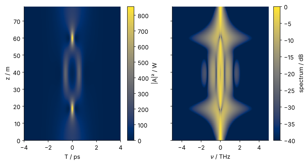
Left: power of a pulse at three times the soliton amplitude over time and distance, narrowing to a bright spike near 18 m and 60 m and back to its input shape at 78.5 m. Right: its spectrum in dB, broadening with fringes at the same distances.

The figure shows the harder case, three times the soliton amplitude, which narrows, splits, and re-forms after 78.5 m; Step 6 draws it. FFTs and frequency grids come from the Fourier transform tutorial, the exact linear step from the KdV tutorial.

Setup

Distances are in m, times in ps, powers in W, so β₂ is in ps²/m and γ in 1/(W m). One grid of 2048 points over 100 ps serves every run.

import numpy as np
import matplotlib.pyplot as plt
from numpy.fft import fft, ifft, fftfreq

beta2 = -20e-3                       # ps^2/m, that is -20 ps^2/km: anomalous
gamma = 1.3e-3                       # 1/(W m)
T0 = 1.0                             # ps
L_D = T0**2 / abs(beta2)             # dispersion length, m
P0 = abs(beta2) / (gamma * T0**2)    # peak power of the fundamental soliton, W
z0 = np.pi / 2 * L_D                 # period of the higher-order solitons, m

N, T_win = 2048, 100.0               # grid points, window in ps
dT = T_win / N
T = (np.arange(N) - N // 2) * dT     # periodic: no point at +T_win/2

plt.rcParams.update({
    "figure.figsize": (7, 3.6), "figure.dpi": 110,
    "axes.spines.top": False, "axes.spines.right": False,
    "axes.grid": True, "grid.alpha": 0.25,
    "font.size": 11, "lines.linewidth": 1.8,
})
INK, ACCENT, SECOND, MUTED = "#1f2a44", "#c8553d", "#2a7f9e", "#8a8f98"

print(f"L_D = {L_D:.1f} m, P0 = {P0:.2f} W, z0 = {z0:.1f} m, dT = {dT * 1e3:.1f} fs")

L_D = 50.0 m, P0 = 15.38 W, z0 = 78.5 m, dT = 48.8 fs

Step 1: Put the pulse on a time grid and its spectrum on a frequency grid

The roles are those of KdV with new names. z, the distance along the fiber, is the evolution variable, as t was; T is the grid coordinate, as x was. The grid is periodic, without its right endpoint, centered on the pulse, and 2π fftfreq gives the angular frequencies in rad/ps.

A convention question comes with every FFT, and half of it does not matter here. A second derivative becomes \(-\omega^2\) for either sign of the exponent in the transform, so the dispersion factor is the same in every book. What does depend on the sign is any odd power of ω and the direction of the frequency axis; this tutorial meets that only when it plots a spectrum, in Step 6.

The cell makes three checks: the energy \(\sum|A|^2\Delta T\) against the exact \(2P_0T_0\), the spectrum in the outer tenth of the frequency grid, and the field at the window's edge. The last two must be negligible, or the pulse wraps around.

omega = 2 * np.pi * fftfreq(N, dT)          # rad/ps, in NumPy's order: 0, positive, negative

A = np.sqrt(P0) / np.cosh(T / T0)
energy = np.sum(np.abs(A)**2) * dT          # W ps = pJ
spec = np.abs(fft(A))
outer = np.abs(omega) > 0.9 * omega.max()
print(f"energy {energy:.3f} pJ, 2 P0 T0 = {2 * P0 * T0:.3f} pJ")
print(f"highest frequency {omega.max():.1f} rad/ps; outer tenth of the spectrum: {spec[outer].max() / spec.max():.0e} of its peak")
print(f"|A| at the window's edge: {np.abs(A[0]) / np.sqrt(P0):.0e} of the peak")

energy 30.769 pJ, 2 P0 T0 = 30.769 pJ
highest frequency 64.3 rad/ps; outer tenth of the spectrum: 7e-17 of its peak
|A| at the window's edge: 4e-22 of the peak

The energy matches \(2P_0T_0\) to the digits printed. In the outer tenth of the frequency grid the spectrum is down to rounding, 7 × 10⁻¹⁷ of its peak, and the pulse's tail at the window's edge, sech(50), is 4 × 10⁻²² of its peak, so nothing wraps around in either direction.

Step 2: Dispersion alone: check against the spreading of a Gaussian pulse

With the Kerr term off, each frequency evolves on its own: \(\partial_T^2 \to -\omega^2\) turns the equation into \(\partial_z \hat A = \tfrac{i}{2}\beta_2\omega^2 \hat A\), so \(\hat A(z + h) = e^{i\beta_2\omega^2 h/2}\,\hat A(z)\), exact for any h. A Gaussian has an exact answer to check it against,

\[A(z, T) = \frac{T_0}{\sqrt{T_0^2 - i\beta_2 z}}\,\exp\!\left(-\frac{T^2}{2\,(T_0^2 - i\beta_2 z)}\right),\]

whose width parameter grows as \(T_0\sqrt{1 + (z/L_D)^2}\), to \(\sqrt{17}\,T_0\) = 4.12 ps at \(z = 4L_D\). One step of 200 m takes it there:

def disperse(A, h, beta2=beta2):
    """Dispersion alone over a length h, exact for any h."""
    return ifft(np.exp(0.5j * beta2 * omega**2 * h) * fft(A))

def gaussian(z, beta2=beta2):
    q = T0**2 - 1j * beta2 * z
    return T0 / np.sqrt(q) * np.exp(-T**2 / (2 * q))

def width(A):
    """The T0 of a Gaussian with the same rms width."""
    I = np.abs(A)**2
    return np.sqrt(2 * np.sum(T**2 * I) / np.sum(I))

z = 4 * L_D
for b2 in [beta2, -beta2]:
    G = disperse(gaussian(0), z, beta2=b2)
    print(f"beta2 = {b2 * 1e3:+.0f} ps^2/km: width {width(G):.4f} ps, "
          f"largest error of the field {np.abs(G - gaussian(z)).max():.1e}")

beta2 = -20 ps^2/km: width 4.1231 ps, largest error of the field 1.7e-16
beta2 = +20 ps^2/km: width 4.1231 ps, largest error of the field 6.1e-01

With the right sign the field agrees with the formula to rounding, 2 × 10⁻¹⁶. With the sign flipped the width is still 4.1231 ps, because the width does not depend on the sign of β₂, but the chirp does, and the field is off by 0.61. Check a dispersion step against the complex field, never against a width alone.

fig, ax = plt.subplots()
for zk, alpha in [(0, 0.35), (L_D, 0.6), (4 * L_D, 0.9)]:
    ax.plot(T, np.abs(disperse(gaussian(0), zk))**2, color=ACCENT, alpha=alpha, lw=4.5)   # wide, so the exact curve shows inside it
    ax.plot(T, np.abs(gaussian(zk))**2, color=INK, lw=1, ls="--")
    T1 = T0 * np.sqrt(1 + (zk / L_D)**2)                  # width parameter at zk
    ax.text(1.3 * T1, 0.75 * np.abs(gaussian(zk)[N // 2])**2, f"z = {zk:.0f} m", color=ACCENT)
ax.text(-11.5, 0.98, "split-step (wide)", color=ACCENT)
ax.text(-11.5, 0.86, "exact (dashed)", color=INK)
ax.set(xlabel="T / ps", ylabel="|A|² / P(0)", xlim=(-12, 12), ylim=(0, 1.12))
plt.show()

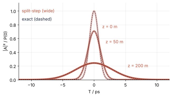
Power of a Gaussian pulse relative to its input peak, against T in ps, at z = 0, 50 m, and 200 m. Wide lines: split-step dispersion step. Dashed: exact formula, inside each wide line. The pulse widens and its peak falls to a quarter.

The peak falls as \(1/\sqrt{1 + (z/L_D)^2}\), to 0.24 of the input at 200 m, and each dashed exact curve lies inside its wide computed one.

Step 3: Add the Kerr effect and propagate the soliton

With dispersion off, the equation is \(\partial_z A = i\gamma|A|^2A\), and \(|A|\) does not change, so \(A(z + h) = A\,e^{i\gamma|A|^2h}\), exact again. Call the two terms of the right-hand side D and N, so that the two exact steps over h are \(e^{hD}\) and \(e^{hN}\), and the true step is \(e^{h(D+N)}\). Expand each exponential to second order: \(e^{hD}e^{hN}\), N first, has the cross term \(h^2DN\) where \(e^{h(D+N)}\) has \((h^2/2)(DN + ND)\), so it misses by \((h^2/2)[D, N]\), with the commutator \([D, N] = DN - ND\). The two do not commute, and over \(L/h\) steps these errors add up to one proportional to h: the first-order, or Lie, splitting. In the symmetric step \(e^{hD/2}e^{hN}e^{hD/2}\) the cross terms come out as \((h^2/2)(DN + ND)\), so one step errs by \(h^3\) and the whole run by \(h^2\): the Strang splitting. This is a statement for small h, and Step 4 shows where it starts to hold.

Two half steps of D in a row are one full step, so the Strang loop costs no more than the Lie loop: one half step at the start, full steps in between, and the last half step undone at the end. The cell runs the soliton over 1 km, the same pulse without the Kerr effect, and finds where that one has doubled its rms width.

def split_step(A, L, h, gamma=gamma, beta2=beta2, order=2):
    """Propagate A over a length L in steps h: order 2 is Strang, order 1 is Lie (N, then D)."""
    half = np.exp(0.25j * beta2 * omega**2 * h)        # dispersion over h/2
    Ah = fft(A) * half if order == 2 else fft(A)
    for _ in range(round(L / h)):
        A = ifft(Ah)
        A = A * np.exp(1j * gamma * np.abs(A)**2 * h)  # Kerr step
        Ah = fft(A) * half**2                          # dispersion step; half steps merged
    return ifft(Ah / half if order == 2 else Ah)

A0 = np.sqrt(P0) / np.cosh(T / T0)
A_kerr = split_step(A0, 1000.0, 1.0)
A_lin = split_step(A0, 1000.0, 1.0, gamma=0.0)
E = lambda A: np.sum(np.abs(A)**2) * dT
print(f"peak power after 1 km: {np.abs(A_kerr).max()**2:.2f} W with the Kerr effect, "
      f"{np.abs(A_lin).max()**2:.2f} W without; at the input {P0:.2f} W")
print(f"energy: input {E(A0):.12f} pJ, after 1 km {E(A_kerr):.12f} pJ")
z_lin = np.arange(0, 300, 0.5)                     # m; dispersion alone, exact at every z
w_lin = [width(disperse(A0, zk)) for zk in z_lin]
print(f"rms width doubled without the Kerr effect at z = {np.interp(2 * width(A0), w_lin, z_lin):.0f} m")

peak power after 1 km: 15.38 W with the Kerr effect, 1.19 W without; at the input 15.38 W
energy: input 30.769230769231 pJ, after 1 km 30.769230769235 pJ
rms width doubled without the Kerr effect at z = 136 m

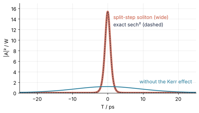
With the Kerr effect the peak is still 15.38 W after 1 km, twenty dispersion lengths; without it the pulse has spread to 1.19 W, its rms width doubled by 136 m. The energy holds to twelve digits, because both factors have modulus 1 and so each step keeps \(\sum|A|^2\Delta T\) fixed. That also means energy says nothing about accuracy: it would be conserved by a step of 100 m.

fig, ax = plt.subplots()
ax.plot(T, np.abs(A_kerr)**2, color=ACCENT, lw=4.5, alpha=0.8)   # wide, so the exact curve shows inside it
ax.plot(T, np.abs(A0)**2, color=INK, lw=1, ls="--")
ax.plot(T, np.abs(A_lin)**2, color=SECOND)
ax.text(1.6, 14, "split-step soliton (wide)", color=ACCENT)
ax.text(1.6, 12.6, "exact sech² (dashed)", color=INK)
ax.text(9, 1.8, "without the Kerr effect", color=SECOND)
ax.set(xlabel="T / ps", ylabel="|A|² / W", xlim=(-25, 25), ylim=(0, 17))
plt.show()

Power against T in ps after 1 km. The wide split-step soliton holds the dashed exact sech squared inside it, at 15.4 W peak; the same pulse without the Kerr effect has spread into a low, broad hump of 1.2 W.

Step 4: Measure the error as the step shrinks

Step 3 predicts slopes of 1 and 2 on a log-log plot of the error against h. The exact soliton, \(A = \sqrt{P_0}\,\mathrm{sech}(T/T_0)\,e^{iz/2L_D}\), gives the error with its phase, as the largest \(|A - A_{\text{exact}}|\) after 1 km relative to \(\sqrt{P_0}\):

h_list = L_D / np.array([5, 10, 20, 50, 100, 200])      # 10 m down to 0.25 m
A_exact = A0 * np.exp(1j * 1000.0 / (2 * L_D))
err = {order: np.array([np.abs(split_step(A0, 1000.0, h, order=order) - A_exact).max()
                        for h in h_list]) / np.sqrt(P0)
       for order in (1, 2)}
print("  h / m   Lie       Strang")
for h, e1, e2 in zip(h_list, err[1], err[2]):
    print(f"{h:7.2f}   {e1:.2e}  {e2:.2e}")

  h / m   Lie       Strang
  10.00   9.14e-02  6.98e-02
   5.00   2.34e-02  1.78e-02
   2.50   6.80e-03  4.48e-03
   1.00   3.49e-03  7.17e-04
   0.50   1.88e-03  1.79e-04
   0.25   9.75e-04  4.48e-05

fig, ax = plt.subplots()
ax.loglog(h_list, err[1], "o-", color=SECOND, ms=6)
ax.loglog(h_list, err[2], "o-", color=ACCENT, ms=6)
h_key = np.array([3.0, 10.0])                                      # a key of the two slopes, in the empty corner
for p, label in [(1, "∝ h"), (2, "∝ h²")]:
    ax.loglog(h_key, 1e-4 * (h_key / h_key[0])**p, color=MUTED, lw=1, ls="--")
    ax.text(h_key[1] * 1.08, 1e-4 * (h_key[1] / h_key[0])**p, label, color=MUTED, va="center")
ax.axvline(1.0, color=MUTED, lw=1, ls="--")                       # the step of the opening question
sup = str.maketrans("-0123456789", "⁻⁰¹²³⁴⁵⁶⁷⁸⁹")
def sci(x):
    mant, expo = f"{x:.1e}".split("e")
    return f"{mant} × 10{str(int(expo)).translate(sup)}"
i1 = np.argmin(np.abs(h_list - 1.0))
ax.text(0.92, err[1][i1] * 1.7, sci(err[1][i1]), color=SECOND, ha="right")
ax.text(1.12, err[2][i1] * 0.55, sci(err[2][i1]), color=ACCENT)
ax.text(0.3, err[1][-1] * 1.8, "Lie", color=SECOND)
ax.text(0.42, err[2][-1] * 1.3, "Strang", color=ACCENT)
ax.set(xlabel="step h / m", ylabel="error / √P₀", xlim=(0.2, 16))
plt.show()

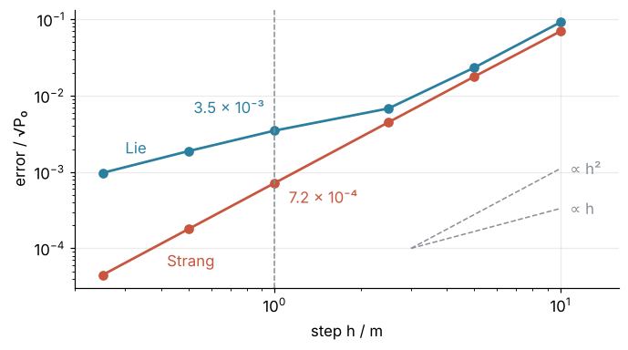
Error of the soliton after 1 km relative to the square root of P0, against the step h in m, log-log. Lie splitting runs parallel to the slope-1 key below 1 m, Strang parallel to the slope-2 key throughout and lower. A dashed line marks h = 1 m, with errors 3.5 × 10⁻³ for Lie and 7.2 × 10⁻⁴ for Strang.

Strang's error falls fourfold per halving of h over the whole table. Lie's falls by a factor of 1.9 per halving below 1 m, and is five times Strang's at 1 m and 22 times at 0.25 m. At h = 1 m the answer to the opening question is 7.2 × 10⁻⁴ of \(\sqrt{P_0}\) for Strang against 3.5 × 10⁻³ for Lie, for the same number of FFTs. Use the symmetric split; there is no reason not to.

Step 5: Choose the step and the window without an exact answer

Start at three times the soliton amplitude, \(A_0 = 3\sqrt{P_0}\,\mathrm{sech}(T/T_0)\), 138 W at the peak: the third-order soliton, which re-forms after \(z_0\) = 78.5 m and has no exact field in between. The step is set by the shortest length in the problem, here \(L_{NL}\) at the highest power, not \(L_D\), and a tenth of it is a good start. That power is unknown before the run, so guess 0.5 m, about a tenth of the input's 5.6 m, and let two checks decide.

Halve the step. Run at h and h/2 and take the largest change of \(|A|\) relative to the input peak. Once Strang's \(h^2\) holds, the error at h/2 is a quarter of that at h, so the change is three quarters of the error at h.

Watch the window's edges. What reaches one edge of a periodic grid comes back in at the other. Take the fraction of the energy in the outer fifth, \(|T| > 0.4\,T_{\text{win}}\), at every stored position along z, and keep the largest.

def edge_fraction(A, T=T):
    I = np.abs(A)**2
    return I[np.abs(T) > 0.4 * len(T) * (T[1] - T[0])].sum() / I.sum()

A3 = 3 * A0
peak = np.abs(A3).max()
runs = {h: split_step(A3, z0, h) for h in [1.0, 0.5, 0.25, z0 / 1000, z0 / 2000]}
for h in [1.0, 0.5]:
    change = np.abs(np.abs(runs[h]) - np.abs(runs[h / 2])).max() / peak
    print(f"halving from h = {h * 100:3.0f} cm: change {change:.1e} of the peak")

A, P_guess = A3, peak**2
for _ in range(round(z0 / 0.5)):               # the guess once more, step by step, to see how high the peak gets
    A = split_step(A, 0.5, 0.5)
    P_guess = max(P_guess, np.abs(A).max()**2)
print(f"peak power at h = 50 cm: {P_guess:.0f} W, so L_NL = {1 / (gamma * P_guess):.2f} m")

halving from h = 100 cm: change 6.3e-02 of the peak
halving from h =  50 cm: change 1.5e-02 of the peak
peak power at h = 50 cm: 848 W, so L_NL = 0.91 m

Halving from the guess changes the pulse by 1.5 % of its peak, a quarter of the 6.3 % from 1 m: the \(h^2\) behavior holds, and both steps are too coarse. In the guess run the pulse compresses to 848 W, which shortens \(L_{NL}\) to 0.91 m, and a tenth of that is 9 cm. Take \(z_0/1000\) = 7.9 cm, just below it, which puts 200 stored positions five steps apart:

h = z0 / 1000
change = np.abs(np.abs(runs[h]) - np.abs(runs[h / 2])).max() / peak
print(f"halving from h = {h * 100:.1f} cm: change {change:.1e} of the peak")

zs = np.linspace(0, z0, 201)
fields = [A3]
for _ in range(200):
    fields.append(split_step(fields[-1], z0 / 200, h))
fields = np.array(fields)
power = np.abs(fields)**2
spectra = np.abs(np.fft.fftshift(fft(fields, axis=1), axes=1))**2

print(f"largest edge fraction along z: {max(edge_fraction(a) for a in fields):.0e}")
for part in [slice(0, 101), slice(100, 201)]:                # the first and the second half of the period
    i = part.start + power[part].max(axis=1).argmax()
    print(f"peak power {power[i].max():.0f} W at z = {zs[i]:.1f} m")
print(f"Kerr phase per step at the peak: {gamma * power.max() * h:.3f} rad")
print(f"return error |A(z0)| against |A0|: {np.abs(np.abs(fields[-1]) - np.abs(A3)).max() / peak:.1e}")

halving from h = 7.9 cm: change 4.4e-04 of the peak
largest edge fraction along z: 3e-21
peak power 856 W at z = 18.5 m
peak power 856 W at z = 60.1 m
Kerr phase per step at the peak: 0.087 rad
return error |A(z0)| against |A0|: 5.9e-04

The change is now 4.4 × 10⁻⁴, and the peak, 856 W at 18.5 m and again at 60.1 m, is within 1 % of the guess run's. Here theory allows one more check: the pulse returns to its input shape within 5.9 × 10⁻⁴ of the peak, and 4.4 × 10⁻⁴ is three quarters of that.

The edge fraction's square root is an amplitude, a rough estimate of the error that wrapping can cause; the second pitfall measures how rough. Keep the fraction below the square of the accuracy you want, 10⁻⁸ for 10⁻⁴. At 3 × 10⁻²¹ this window has room to spare.

Step 6: Draw the intensity and the spectrum against distance

The light is the carrier times A. With the carrier written \(e^{-i\omega_0 t}\), as in Agrawal, and A built by ifft from \(e^{+i\omega T}\), a component at ω oscillates at \(\omega_0 - \omega\), so NumPy's positive frequencies lie below the carrier. The spectrum goes against \(\nu = -\)fftfreq in THz, the offset from the carrier's 193.4 THz. For this symmetric spectrum the choice only decides which side is blue.

nu = -np.fft.fftshift(fftfreq(N, dT))                     # THz, offset from the carrier
spec_dB = 10 * np.log10(spectra / spectra[0].max() + 1e-12)   # floor at -120 dB: some bins are exactly 0

fig, (ax1, ax2) = plt.subplots(1, 2, figsize=(8, 4.2), sharey=True, layout="constrained")
fig.get_layout_engine().set(wspace=0.08)                  # room between the left colorbar's label and the right panel
im1 = ax1.pcolormesh(T, zs, power, cmap="cividis", shading="auto", rasterized=True)
im2 = ax2.pcolormesh(nu, zs, spec_dB, cmap="cividis", shading="auto", vmin=-40, vmax=0, rasterized=True)
fig.colorbar(im1, ax=ax1, label="|A|² / W")
fig.colorbar(im2, ax=ax2, label="spectrum / dB")
ax1.set(xlabel="T / ps", ylabel="z / m", xlim=(-4, 4), ylim=(0, z0))
ax2.set(xlabel="$\\nu$ / THz", xlim=(-5, 5), xticks=[-4, -2, 0, 2, 4])
for ax in (ax1, ax2):
    ax.grid(False)
plt.show()

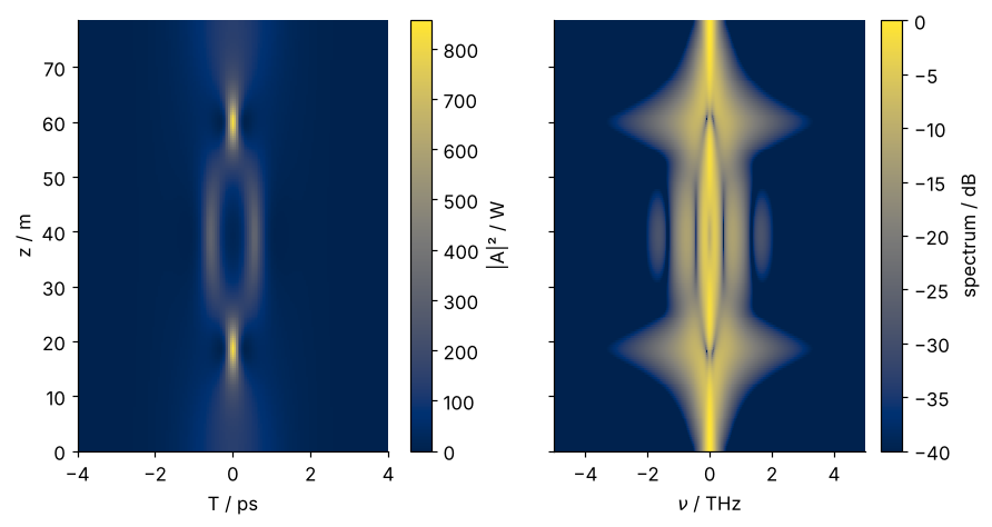
Left: power of the third-order soliton in W over T in ps and z in m, cividis colors, a single pulse that narrows to a bright spike near 18 m and 60 m, splits into two near 39 m, and returns at 78.5 m. Right: the spectrum in dB over frequency offset in THz and z, broadest at the same distances.

Where the pulse narrows to a spike, near 18 m and 60 m, the spectrum is broadest and grows fringes; at 39 m the pulse splits in two and the spectrum narrows to a central peak with side lobes. At 78.5 m both are back to the input.

Pitfalls

The wrong sign in the dispersion factor. Engineering texts write the oscillation as \(e^{j\omega t}\), so their \(j\) is this tutorial's \(-i\) and their dispersion step reads \(e^{-j\beta_2\omega^2h/2}\). Copy it with \(j\) read as \(i\), keep this tutorial's Kerr step, and the soliton falls apart:

A_flip = split_step(A0, 1000.0, 1.0, beta2=-beta2)        # the same as flipping the factor's sign
print(f"peak power after 1 km with the flipped sign: {np.abs(A_flip).max()**2:.2f} W (correct: {P0:.2f} W)")

peak power after 1 km with the flipped sign: 0.65 W (correct: 15.38 W)

At the soliton power it spreads to 0.65 W, faster than without the Kerr effect at all, because the flipped factor is normal dispersion, whose chirp adds to the Kerr chirp. Derive the factor from \(\partial_T^2 \to -\omega^2\) and run Step 2's check on the complex field.

A time window that is too small. A Gaussian spread to 20 \(L_D\) is about 20 ps wide. Put it in windows of 50, 100, and 200 ps at the same ΔT:

for T_w in [50.0, 100.0, 200.0]:
    n = round(T_w / dT)
    Tw = (np.arange(n) - n // 2) * dT
    om = 2 * np.pi * fftfreq(n, dT)
    G0 = np.exp(-Tw**2 / (2 * T0**2))
    q = T0**2 - 1j * beta2 * 20 * L_D
    G = ifft(np.exp(0.5j * beta2 * om**2 * 20 * L_D) * fft(G0))
    G_exact = T0 / np.sqrt(q) * np.exp(-Tw**2 / (2 * q))
    f = edge_fraction(G, Tw)
    e = np.abs(G - G_exact).max() / np.abs(G_exact).max()
    print(f"window {T_w:3.0f} ps: edge fraction {f:.1e}, its square root {np.sqrt(f):.1e}, "
          f"error {e:.1e} of the peak, ratio {np.sqrt(f) / e:5.2f}")

window  50 ps: edge fraction 1.2e-01, its square root 3.5e-01, error 4.6e-01 of the peak, ratio  0.76
window 100 ps: edge fraction 4.7e-03, its square root 6.8e-02, error 4.4e-02 of the peak, ratio  1.54
window 200 ps: edge fraction 1.6e-08, its square root 1.3e-04, error 3.8e-06 of the peak, ratio 32.93

At 50 ps 12 % of the energy sits in the outer fifth and the field is off by 46 % of its peak; the tails have come back in at the other side. At 100 ps the edge fraction is 0.5 % and the error 4 %; at 200 ps, 1.6 × 10⁻⁸ and 4 × 10⁻⁶. The edge fraction tells you this without the exact field. Its square root lands within a factor of two of the error in the two narrow windows, 0.76 and 1.54 times it, and overestimates it by a factor of 33 in the wide one, which is the safe side. Widen the window at fixed ΔT until the fraction is below the square of your accuracy.

A step chosen from the dispersion length alone. h = 1 m, a fiftieth of \(L_D\), gives the fundamental soliton an error of 7 × 10⁻⁴ (Step 4), but not the third-order soliton:

print(f"third-order soliton at h = 1 m: return error {np.abs(np.abs(runs[1.0]) - np.abs(A3)).max() / peak:.1e} of the peak")

third-order soliton at h = 1 m: return error 8.2e-02 of the peak

Its peak power shortens \(L_{NL}\) to 0.9 m (Step 5), and the halving check flags it without the exact answer: halving from 1 m changed the pulse by 6.3 %, three quarters of this 8.2 %. Either halve until the change is small enough, or use an adaptive step that keeps the Kerr phase \(\gamma|A|^2h\) per step below a bound, which the production run of Step 5 kept under 0.09 rad.

Variations

Fiber loss or gain. Add \(-\alpha/2\) to the dispersion step's exponent, \(e^{(i\beta_2\omega^2/2 - \alpha/2)h}\); the soliton then broadens as its power drops.
Third-order dispersion. Add \(-i\beta_3\omega^3h/6\) to the exponent. \(\omega^3\) is odd, so here the sign of the transform matters (Step 1), and the soliton sheds radiation to one side.
Normal dispersion, β₂ > 0. There is no bright soliton. A strong pulse broadens faster than by dispersion alone, and its edges break into ripples where its fast and slow parts overtake each other, which is called optical wave breaking.
A beam instead of a pulse. Transverse coordinates replace T and the angular spectrum propagator replaces the dispersion step: the beam propagation method, whose linear step is the angular spectrum method with numpy.fft.

Cheat sheet

T = (np.arange(N) - N//2) * dT                    # periodic, no endpoint
omega = 2*np.pi*fftfreq(N, dT)                    # rad per unit of T
half = np.exp(0.25j*beta2*omega**2*h)             # ∂T² -> -ω², dispersion over h/2
Ah = fft(A) * half                                # Strang: first half step
for _ in range(round(L/h)):
    A = ifft(Ah); A = A*np.exp(1j*gamma*np.abs(A)**2*h)   # Kerr step, exact
    Ah = fft(A) * half**2                         # two half steps merged
A = ifft(Ah / half)                               # undo the extra half step
# check: rerun at h/2 (change ~ 3/4 of the error), edge fraction < accuracy²