Crank-Nicolson for the Schrödinger equation: tunneling through a barrier (Python)

The problem: how much of an electron tunnels through a barrier?

An electron with a mean energy of 4.93 eV runs at a barrier 6.80 eV high and 0.21 nm wide. A classical particle with that energy bounces back every time. The electron does not: 16.2 % of it comes out on the other side. That is tunneling, the effect a scanning tunneling microscope measures and the reason alpha decay happens at all.

The electron is described by a complex wave function \(\psi(x, t)\) that obeys the time-dependent Schrödinger equation

\[i\hbar\,\frac{\partial\psi}{\partial t} = -\frac{\hbar^2}{2m}\frac{\partial^2\psi}{\partial x^2} + V(x)\,\psi ,\]

with \(V(x)\) the barrier. \(|\psi|^2\,dx\) is the probability of finding the electron in \(dx\), so \(\int|\psi|^2\,dx = 1\) must hold at all times. The code uses atomic units, \(\hbar = m = 1\) with \(m\) the electron mass: length in bohr (0.0529 nm), energy in hartree (27.2 eV), time in units of 24.2 as.

The method is Crank-Nicolson: one sparse linear solve per time step, and the total probability stays at 1 however large the step. Step 6 draws this figure:

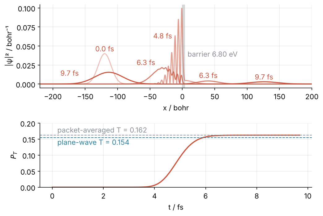
Top: probability density of the electron against x in bohr at four times, with the barrier as a gray band; the packet arrives from the left, forms fringes at the barrier, and splits. Bottom: transmitted probability against time in fs, leveling off at 0.162, above the plane-wave value 0.154.

The packet arrives, piles up in fringes in front of the barrier, and splits. The transmitted part levels off at 0.162, 5 % above the 0.154 that the textbook transmission coefficient gives at the mean energy, and Step 6 shows where the difference comes from.

Setup

import warnings

import numpy as np
import scipy.sparse as sparse
from scipy.sparse.linalg import splu
import matplotlib.pyplot as plt

HARTREE_EV = 27.211386   # eV per hartree
BOHR_NM = 0.052917721    # nm per bohr
AU_FS = 0.024188843      # fs per atomic unit of time

k0, sigma, x0 = 0.6, 10.0, -120.0   # mean wavenumber / bohr⁻¹, packet width / bohr, start / bohr
V0, a = 0.25, 4.0                   # barrier height / hartree, width / bohr
L = 300.0                           # the domain runs from -L to L, bohr

plt.rcParams.update({                      # the look of every figure below
    "figure.figsize": (7, 3.6), "figure.dpi": 110,
    "axes.spines.top": False, "axes.spines.right": False,
    "axes.grid": True, "grid.alpha": 0.25,
    "font.size": 11, "lines.linewidth": 1.8,
})
INK, ACCENT, SECOND, MUTED = "#1f2a44", "#c8553d", "#2a7f9e", "#8a8f98"

print(f"mean energy {(k0**2 / 2 + 1 / (8 * sigma**2)) * HARTREE_EV:.2f} eV, barrier {V0 * HARTREE_EV:.2f} eV, "
      f"width {a * BOHR_NM:.3f} nm")

mean energy 4.93 eV, barrier 6.80 eV, width 0.212 nm

Step 1: Put the wave packet and the barrier on a grid

The packet is a Gaussian envelope of width \(\sigma\) times the factor \(e^{ik_0x}\), a plane wave that gives it momentum \(p = \hbar k_0\) and makes it move to the right. Here \(\sigma\) is the rms width of \(|\psi|^2 \propto e^{-(x-x_0)^2/(2\sigma^2)}\), the spread in position. Normalize it so that the sum of \(|\psi|^2\Delta x\) is 1:

def grid(dx):
    return np.linspace(-L, L, round(2 * L / dx) + 1)

def potential(x):
    # your own V(x) goes here; the barrier covers 0 <= x < a
    return np.where((x >= 0) & (x < a), V0, 0.0)

def packet(x, sigma=sigma):
    psi = np.exp(-(x - x0)**2 / (4 * sigma**2) + 1j * k0 * x)
    return psi / np.sqrt(np.sum(np.abs(psi)**2) * (x[1] - x[0]))

dx = 0.1
x = grid(dx)
psi0 = packet(x)
print(f"{x.size} points, {2 * np.pi / k0 / dx:.0f} per wavelength")
print(f"norm {np.sum(np.abs(psi0)**2) * dx:.12f}")
print(f"largest |psi|^2 at the edges {np.abs(psi0[np.abs(x) > L - 20]).max()**2:.1e}, "
      f"in the barrier {np.abs(psi0[potential(x) > 0]).max()**2:.1e}")

6001 points, 105 per wavelength
norm 1.000000000000
largest |psi|^2 at the edges 8.7e-58, in the barrier 2.1e-33

A wavelength \(2\pi/k_0\) spans 105 grid points, and at \(t = 0\) the packet is nowhere near the barrier or the walls.

Step 2: Build the Hamiltonian as a sparse matrix

The right-hand side of the Schrödinger equation is a matrix \(H\) applied to \(\psi\), the Hamiltonian. Its kinetic part is \(-\tfrac12\) times the second difference \((\psi_{j-1} - 2\psi_j + \psi_{j+1})/\Delta x^2\), as in Finite differences: the heat equation as a matrix, and \(V\) adds to the diagonal. That is three diagonals, so sparse.diags_array builds it, in CSC format for reasons Step 3 gives. Cutting the matrix off at the ends sets \(\psi = 0\) beyond them: hard walls.

def hamiltonian(x):
    dx = x[1] - x[0]
    off = np.full(x.size - 1, -0.5 / dx**2)
    return sparse.diags_array([off, 1 / dx**2 + potential(x), off],
                              offsets=[-1, 0, 1], format="csc")

H = hamiltonian(x)
E_mean = np.real(np.sum(np.conj(psi0) * (H @ psi0))) * dx
print(f"nonzeros {H.nnz}, largest |H - H^†| = {abs(H - H.conj().T).max()}")
print(f"mean energy {E_mean:.5f} hartree, continuum value {k0**2 / 2 + 1 / (8 * sigma**2):.5f}")

nonzeros 18001, largest |H - H^†| = 0.0
mean energy 0.18119 hartree, continuum value 0.18125

\(H\) equals its conjugate transpose exactly, and that symmetry is what keeps the total probability at 1 in Step 3. The sum \(\sum_j \psi_j^* (H\psi)_j\,\Delta x\) is the energy averaged over the packet: 0.18119 hartree on the grid against 0.18125 in the continuum, where the \(1/(8\sigma^2)\) comes from the envelope. It is below \(V_0 = 0.25\), so classically the whole packet is reflected.

Step 3: Step with Crank-Nicolson, the average of explicit and implicit Euler

In atomic units the equation is \(\partial\psi/\partial t = -iH\psi\). Explicit Euler evaluates \(H\psi\) at the old time, \(\psi^{n+1} = (I - i\Delta t H)\psi^n\). Implicit Euler evaluates it at the new time, \((I + i\Delta t H)\psi^{n+1} = \psi^n\). Crank-Nicolson takes half of each:

\[\left(I + \tfrac{i\Delta t}{2}H\right)\psi^{n+1} = \left(I - \tfrac{i\Delta t}{2}H\right)\psi^n .\]

Any \(\psi\) is a sum of eigenvectors \(v\) of \(H\), \(Hv = Ev\), each a state of definite energy \(E\). Because \(H\) is Hermitian, the \(E\) are real and the \(v\) orthogonal, so the norm of \(\psi\) is the sum of the squared sizes of its parts. The exact equation turns each part by the phase \(e^{-iE\Delta t}\) per step. Crank-Nicolson multiplies it by \((1 - i\Delta tE/2)/(1 + i\Delta tE/2)\), a ratio of two complex conjugates, of modulus exactly 1 for every real \(E\) and every \(\Delta t\), so the norm stays at 1. Explicit Euler multiplies it by \(1 - i\Delta tE\), of modulus \(\sqrt{1 + \Delta t^2E^2} > 1\):

dt = 0.5
psi = psi0.copy()
for n in range(1, 11):
    psi = psi - 1j * dt * (H @ psi)
    if n in (1, 5, 10):
        print(f"explicit Euler, {n:2d} steps: norm {np.sum(np.abs(psi)**2) * dx:.4g}")

explicit Euler,  1 steps: norm 1.008
explicit Euler,  5 steps: norm 1.043
explicit Euler, 10 steps: norm 1.698e+10

Ten steps, and the norm is \(1.7 \times 10^{10}\). The culprit is the zigzag from one grid point to the next, the largest energy the grid holds (\(2/\Delta x^2 = 200\), Step 5's formula at \(k\Delta x = \pi\)): it grows a hundredfold per step out of rounding noise.

The Crank-Nicolson factor is \(e^{-i\theta}\) with \(\theta = 2\arctan(\Delta tE/2)\), close to \(E\Delta t\) only while \(\Delta tE/2\) is small; Step 5 measures what that lag does. splu does the Gaussian elimination of \(A\) once and keeps a lower and an upper triangle, so each step is two triangular solves. It wants CSC, column-wise storage, hence the format of \(H\):

I = sparse.eye_array(x.size, format="csc")
A = I + 0.5j * dt * H
B = I - 0.5j * dt * H
lu = splu(A)

psi = lu.solve(B @ psi0)
print(f"one Crank-Nicolson step: norm - 1 = {np.sum(np.abs(psi)**2) * dx - 1:.1e}")
print(f"nonzeros: H {H.nnz}, L + U {lu.L.nnz + lu.U.nnz}")

one Crank-Nicolson step: norm - 1 = -2.3e-13
nonzeros: H 18001, L + U 24004

The norm is 1 to rounding. With 24,004 nonzeros in the triangles and 18,001 in \(B\), a step costs about 2.3 products with \(H\).

Step 4: Run the packet into the barrier and measure what gets through

The loop is one line. Every 5 atomic time units it records the transmitted probability \(P_T\), the sum of \(|\psi|^2\Delta x\) beyond the barrier, the reflected \(P_R\) in front of it, the norm, and the center of the transmitted part, which Step 5 needs:

def run(x, psi, dt=0.5, t_end=400.0, snap_times=()):
    dx = x[1] - x[0]
    I = sparse.eye_array(x.size, format="csc")
    H = hamiltonian(x)
    lu, B = splu(I + 0.5j * dt * H), I - 0.5j * dt * H
    every, n_steps = max(1, round(5 / dt)), round(t_end / dt)
    snap_steps = {round(t / dt): t for t in snap_times}
    rec, snaps = {"t": [], "PT": [], "PR": [], "norm": [], "center": []}, {}
    for n in range(n_steps + 1):
        if n % every == 0 or n == n_steps:
            rho = np.abs(psi)**2 * dx
            beyond = x >= a
            rec["t"].append(n * dt)
            rec["PT"].append(rho[beyond].sum())
            rec["PR"].append(rho[x < 0].sum())
            rec["norm"].append(rho.sum())
            rec["center"].append((rho[beyond] * x[beyond]).sum() / rho[beyond].sum())
        if n in snap_steps:
            snaps[snap_steps[n]] = np.abs(psi)**2
        if n < n_steps:
            psi = lu.solve(B @ psi)
    return {key: np.array(val) for key, val in rec.items()}, snaps

main, snaps = run(x, psi0, snap_times=(0, 200, 260, 400))
print("  t / au   t / fs     P_T       P_R    in barrier")
for t in (150, 200, 250, 300, 350, 400):
    i = np.searchsorted(main["t"], t)
    PT, PR = main["PT"][i], main["PR"][i]
    print(f"{t:8.0f} {t * AU_FS:7.2f}  {PT:8.5f}  {PR:8.5f}  {1 - PT - PR:9.2e}")
print(f"largest |norm - 1| over the run: {np.abs(main['norm'] - 1).max():.1e}")

  t / au   t / fs     P_T       P_R    in barrier
     150    3.63   0.00070   0.99526   4.04e-03
     200    4.84   0.07490   0.83372   9.14e-02
     250    6.05   0.15757   0.82883   1.36e-02
     300    7.26   0.16221   0.83757   2.21e-04
     350    8.47   0.16225   0.83774   1.81e-06
     400    9.68   0.16225   0.83775   1.51e-08
largest |norm - 1| over the run: 5.1e-13

At \(t = 200\) about 9 % of the probability sits inside the barrier. From \(t = 350\) on \(P_T\) stands still at 0.16225, \(P_R\) ends at 0.83775, and the norm moves by at most \(5.1 \times 10^{-13}\) in 800 steps. At \(t = 400\) (9.7 fs) both parts are clear of the barrier and still far from the walls.

Step 5: Choose the time step and the grid spacing

Crank-Nicolson is stable at any \(\Delta t\), which tempts you to take big steps. The catch is the phase lag of Step 3. A phase \(\theta\) per step is a frequency \(\omega = \theta/\Delta t\), and a packet moves at the group velocity \(d\omega/dk\). Exact stepping gives \(\theta = E\Delta t\); Crank-Nicolson multiplies every \(d\omega\) by the slope \(d\theta/d(E\Delta t) = 1/(1 + (\Delta tE/2)^2)\), which the code prints at the mean energy:

for dt_try in (0.5, 5.0, 10.0):
    r, _ = run(x, psi0, dt=dt_try)
    slowdown = 1 / (1 + (dt_try * E_mean / 2)**2)
    print(f"dt = {dt_try:4.1f}: P_T(400) = {r['PT'][-1]:.5f}, transmitted center at x = "
          f"{r['center'][-1]:5.1f} bohr, group velocity factor {slowdown:.3f}")

dt =  0.5: P_T(400) = 0.16225, transmitted center at x = 126.0 bohr, group velocity factor 0.998
dt =  5.0: P_T(400) = 0.16225, transmitted center at x =  78.9 bohr, group velocity factor 0.830
dt = 10.0: P_T(400) = 0.09894, transmitted center at x =  16.2 bohr, group velocity factor 0.549

At \(\Delta t = 5\) the transmitted probability is right, but the packet is at \(x = 79\) instead of 126 bohr. At \(\Delta t = 10\) the packet moves at 0.549 of its true speed, has barely left the barrier, and \(P_T\) reads 0.099. Run longer and the large step reaches the same plateau late. It keeps the eigenvectors exact and gets only their phases wrong, so the share of each energy, and with it the share that tunnels, is right:

fine, _ = run(x, psi0, dt=0.5, t_end=800)
coarse, _ = run(x, psi0, dt=10.0, t_end=800)
print(f"P_T at t = 800: dt = 0.5 gives {fine['PT'][-1]:.5f}, dt = 10 gives {coarse['PT'][-1]:.5f}")

fig, ax = plt.subplots()
ax.plot(coarse["t"] * AU_FS, coarse["PT"], "o-", color=SECOND, ms=4)
ax.plot(fine["t"] * AU_FS, fine["PT"], color=ACCENT)     # the run of Steps 4 and 6
ax.text(5.6, 0.12, "Δt = 0.5", color=ACCENT)
ax.text(11.5, 0.12, "Δt = 10", color=SECOND)
ax.set(xlabel="t / fs", ylabel="transmitted probability $P_T$", ylim=(0, 0.18))
plt.show()

P_T at t = 800: dt = 0.5 gives 0.16225, dt = 10 gives 0.16225

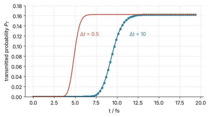
Transmitted probability P_T against time in fs for time steps 0.5 and 10 atomic units. Both curves reach the same plateau of 0.162; the large step gets there about twice as late.

The rule: the result is right once the packet has finished, but times and positions along the way are right only while \(\Delta tE/2\) is small for the energies the packet holds, 0.045 here at the mean energy and \(\Delta t = 0.5\). The grid is the second knob:

for dx_try in (0.05, 0.1, 0.2, 0.5, 1.0):
    x_try = grid(dx_try)
    r, _ = run(x_try, packet(x_try))
    E_grid = (1 - np.cos(k0 * dx_try)) / dx_try**2
    print(f"dx = {dx_try:4.2f}: {2 * np.pi / k0 / dx_try:5.1f} points per wavelength, "
          f"P_T = {r['PT'][-1]:.5f}, kinetic energy at k0 {E_grid:.4f}")

dx = 0.05: 209.4 points per wavelength, P_T = 0.16239, kinetic energy at k0 0.1800
dx = 0.10: 104.7 points per wavelength, P_T = 0.16225, kinetic energy at k0 0.1799
dx = 0.20:  52.4 points per wavelength, P_T = 0.16170, kinetic energy at k0 0.1798
dx = 0.50:  20.9 points per wavelength, P_T = 0.15791, kinetic energy at k0 0.1787
dx = 1.00:  10.5 points per wavelength, P_T = 0.14525, kinetic energy at k0 0.1747

Halving \(\Delta x\) from 0.1 changes \(P_T\) by 0.1 %, so 0.1 is converged. At 52 points per wavelength \(P_T\) is 0.4 % low, at 21 points 3 %, at 10 points 11 %. The second difference sees a plane wave's kinetic energy as \((1 - \cos k\Delta x)/\Delta x^2\), slightly below \(k^2/2\), and tunneling depends exponentially on how far the energy sits below the barrier. Take 50 or more points per wavelength, and halve \(\Delta x\) once to check.

Step 6: Compare with the plane-wave transmission coefficient

The textbook answer is the transmission coefficient \(T\), the fraction of an incoming plane wave of one sharp energy \(E\) that passes the barrier:

\[T(E) = \left[1 + \frac{V_0^2\sinh^2(\kappa a)}{4E(V_0 - E)}\right]^{-1}, \qquad \kappa = \sqrt{2(V_0 - E)} ,\]

with \(\kappa\) the rate at which \(\psi\) decays inside the barrier. Above \(V_0\) the sinh becomes a sine and \(V_0 - E\) becomes \(E - V_0\). The packet, though, is a sum of plane waves, and the Fourier transform of its envelope gives each wavenumber the weight \(|\phi(k)|^2 \propto e^{-2\sigma^2(k - k_0)^2}\). Each plane wave passes the barrier on its own, so average \(T(k^2/2)\) over that:

def transmission(E):
    q = np.sqrt(2 * np.abs(V0 - E))
    s = np.where(E < V0, np.sinh(q * a), np.sin(q * a))
    return 1 / (1 + V0**2 * s**2 / (4 * E * np.abs(V0 - E)))

def averaged_T(sigma):
    k = np.linspace(0.01, 1.5, 3000)
    weight = np.exp(-2 * sigma**2 * (k - k0)**2)
    return np.sum(weight * transmission(k**2 / 2)) / np.sum(weight)

def mean_energy(sigma):
    return k0**2 / 2 + 1 / (8 * sigma**2)

T_mean = transmission(mean_energy(10))
narrow, _ = run(x, packet(x, sigma=5.0))
for s_, r_ in ((10, main), (5, narrow)):
    print(f"sigma = {s_:2d}: run {r_['PT'][-1]:.4f}, T at the mean energy "
          f"{transmission(mean_energy(s_)):.4f}, averaged T {averaged_T(s_):.4f}")

sigma = 10: run 0.1623, T at the mean energy 0.1544, averaged T 0.1624
sigma =  5: run 0.1919, T at the mean energy 0.1618, averaged T 0.1921

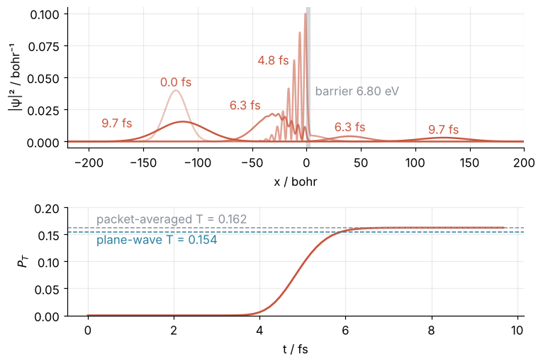
At the mean energy \(T = 0.154\), and the run gives 0.162. The average over the packet's energies gives 0.162 too: \(T\) rises so steeply with energy below the barrier that the faster half of the packet gains more than the slower half loses. Halve the width to \(\sigma = 5\) and the spread of energies doubles. The run reads 0.192, 19 % above the plane-wave \(T\) at this packet's own mean energy (0.162 here, a coincidence with the number above), and the average again reproduces it. The figure from the top puts the snapshots and the transmitted probability together:

fig, (ax1, ax2) = plt.subplots(2, 1, figsize=(7, 4.8), height_ratios=[1.3, 1])
for t, alpha in zip((0, 200, 260, 400), (0.35, 0.55, 0.75, 1.0)):
    ax1.plot(x, snaps[t], color=ACCENT, alpha=alpha, lw=1.6)
ax1.axvspan(0, a, color=MUTED, alpha=0.35, lw=0)
ax1.text(8, 0.036, f"barrier {V0 * HARTREE_EV:.2f} eV", color=MUTED)
for t, xt, yt, ha in ((0, -120, 0.043, "center"), (200, -16, 0.06, "right"),    # a label on each part
                      (260, -42, 0.025, "right"), (260, 40, 0.008, "center"),
                      (400, -160, 0.011, "right"), (400, 126, 0.006, "center")):
    ax1.text(xt, yt, f"{t * AU_FS:.1f} fs", color=ACCENT, ha=ha)
ax1.set(xlabel="x / bohr", ylabel="|ψ|² / bohr⁻¹", xlim=(-220, 200))

ax2.plot(main["t"] * AU_FS, main["PT"], color=ACCENT)
ax2.axhline(T_mean, color=SECOND, lw=1, ls="--")
ax2.axhline(averaged_T(10), color=MUTED, lw=1, ls="--")
ax2.text(0.2, T_mean - 0.022, f"plane-wave T = {T_mean:.3f}", color=SECOND)
ax2.text(0.2, averaged_T(10) + 0.008, f"packet-averaged T = {averaged_T(10):.3f}", color=MUTED)
ax2.set(xlabel="t / fs", ylabel="$P_T$", ylim=(0, 0.2))
fig.tight_layout()
plt.show()

Top: probability density |psi|^2 in 1/bohr against x in bohr at 0, 4.8, 6.3 and 9.7 fs, the barrier a gray band at x = 0 to 4; the packet arrives, forms fringes, and splits. Bottom: transmitted probability against time in fs, leveling off at 0.162 on the packet-averaged T and above the plane-wave T of 0.154 at the mean energy.

Pitfalls

The norm drifts. The sum of \(|\psi|^2\Delta x\) grows or decays steadily, by far more than rounding. The cause is a pair \(A\), \(B\) that is not \(I \pm i\Delta tH/2\): \(\Delta t\) on one side and \(\Delta t/2\) on the other, a sign flipped, or \(V\) added to one matrix only. Forget \(V\) in \(B\) and rerun the 800 steps of Step 4:

K = H - sparse.diags_array(potential(x), format="csc")   # kinetic part only
lu_bad, B_bad = splu(I + 0.5j * dt * H), I - 0.5j * dt * K
psi = psi0.copy()
for n in range(1, 801):
    psi = lu_bad.solve(B_bad @ psi)
    if n in (100, 800):
        print(f"{n:3d} steps: norm {np.sum(np.abs(psi)**2) * dx:.4f}")

100 steps: norm 1.0000
800 steps: norm 0.9031

The norm holds while the packet is far from the barrier, where \(V\) is zero anyway, and ends at 0.90. The factor of Step 3 is no longer a ratio of complex conjugates. Print the norm in every run; it costs one sum and catches every one of these.

Reflection from the wall read as reflection from the barrier. Run the same packet much longer and \(P_T\) keeps changing:

long, _ = run(x, psi0, dt=1.0, t_end=1600)
for t in (400, 1000, 1200, 1400):
    print(f"t = {t:4d} ({t * AU_FS:4.1f} fs): P_T = {long['PT'][np.searchsorted(long['t'], t)]:.3f}")

t =  400 ( 9.7 fs): P_T = 0.162
t = 1000 (24.2 fs): P_T = 0.163
t = 1200 (29.0 fs): P_T = 0.253
t = 1400 (33.9 fs): P_T = 0.285

Both parts bounce off the hard walls, come back, and hit the barrier again, so by \(t = 1{,}400\) more than a quarter sits on the right. Stop the run when both parts are clear of the barrier and still away from the walls, check the probability within 20 bohr of each edge, or widen the domain.

A packet stored in a real array. Fill a preallocated float array with the complex packet and NumPy keeps the real part, with nothing louder than a warning:

psi_real = np.zeros(x.size)
with warnings.catch_warnings(record=True) as caught:
    warnings.simplefilter("always")
    psi_real[:] = np.exp(-(x - x0)**2 / (4 * sigma**2) + 1j * k0 * x)
print(f"{caught[0].category.__name__}: {caught[0].message}")
psi_real /= np.sqrt(np.sum(psi_real**2) * dx)
r, _ = run(x, psi_real.astype(complex))
print(f"P_T = {r['PT'][-1]:.3f}")

ComplexWarning: Casting complex values to real discards the imaginary part
P_T = 0.081

The packet is now a Gaussian times \(\cos k_0x\), two packets running in opposite directions, and only one of them meets the barrier. \(P_T\) reads half the true value. Create \(\psi\) complex from the start, np.zeros(n, dtype=complex) or straight from the complex expression, and check in the first steps that the center moves to the right.

Variations

Any potential. Change potential(x): two barriers in a row for resonant tunneling, a smooth Gaussian bump, or \(k_0\) above \(\sqrt{2V_0}\) for reflection from a barrier the classical particle would cross.
An absorbing edge. Add \(-iW(x)\) to the diagonal near both ends, with \(W\) rising smoothly from 0. The norm then falls on purpose, and what it loses is what left the domain.
A harmonic well. \(V = \tfrac12\omega^2x^2\). A displaced Gaussian oscillates with period \(2\pi/\omega\), a sharp check on the time step.
Two dimensions. Build the Laplacian with sparse.kron as in Poisson's equation with scipy.sparse. splu still works on moderate grids.

Cheat sheet

off = np.full(N - 1, -0.5 / dx**2)                       # kinetic part, hbar = m = 1
H = sparse.diags_array([off, 1 / dx**2 + V, off], offsets=[-1, 0, 1], format="csc")
I = sparse.eye_array(N, format="csc")
A, B = I + 0.5j * dt * H, I - 0.5j * dt * H              # same H, same dt/2 on both sides
lu = splu(A)                                             # factor once; give it CSC
for n in range(n_steps):
    psi = lu.solve(B @ psi)                              # one Crank-Nicolson step
norm = np.sum(np.abs(psi)**2) * dx                       # stays 1; if not, A and B disagree
P_T = np.sum(np.abs(psi[x >= a])**2) * dx                # probability beyond the barrier