Surface temperature of an airless planet in Julia: day, night, and below the ground

The problem: a day and a night on the Moon's equator

Noon returns to the Moon's equator every 29.53 Earth days, with two weeks of sunshine and two weeks of darkness between and no air to hold the warmth. If the ground stored no heat, the surface temperature would follow the Sun alone: 386 K at noon, absolute zero all night. Diviner, the radiometer on NASA's Lunar Reconnaissance Orbiter, records about 95 K just before sunrise. What closes the gap is conduction of heat into the regolith, the broken rock and dust on top, which soaks up heat by day and gives it back after dark.

With the depth \(z\) counted downward, the density \(\rho\), the specific heat \(c\), and the thermal conductivity \(k\), the temperature \(T\) below the surface obeys the heat equation:

\[ \rho c\,\frac{\partial T}{\partial t} = k\,\frac{\partial^2 T}{\partial z^2} . \]

At the surface, sunlight that is absorbed and not radiated back to space has to be conducted downward:

\[ -k\,\frac{\partial T}{\partial z}\Big|_{z=0} = (1 - A)\,S\,\max(\cos h,\, 0) - \varepsilon \sigma T^4 . \]

\(S\) stands for the solar flux and \(A\) for the albedo; \(\varepsilon\sigma T^4\) is thermal emission with the emissivity \(\varepsilon\) and the Stefan-Boltzmann constant \(\sigma\). The angle \(h\) is the Sun's position counted from noon, and the maximum sets the sunlight to zero after sunset. At 1 m the column is closed: no heat crosses it.

The \(T^4\) rules out a textbook solution. Slice the ground into thin layers instead, give each layer one ODE, and hand the set to DifferentialEquations.jl. That is the method of lines, the one thing here the pendulum did not teach.

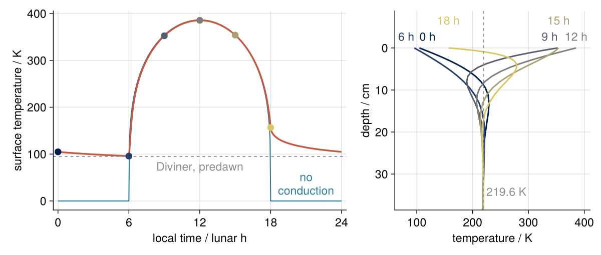
Left: lunar surface temperature in K against local time in lunar hours (one is 29.5 Earth hours). The model stays above the 95 K Diviner line all night, while radiation alone drops to 0 K at sunset. Right: temperature against depth in cm at six times of day; the daily swing dies out within about 30 cm, at 219.6 K.

Left, the surface through one lunar day, with the radiation-only curve and the Diviner value; right, the temperature against depth at six moments of that day. Step 6 draws it.

Setup

The solvers of DifferentialEquations.jl live in OrdinaryDiffEq, and that package is all this tutorial loads; with using DifferentialEquations every line runs unchanged. Install the two packages once with import Pkg; Pkg.add(["OrdinaryDiffEq", "CairoMakie"]). Printf and Statistics come with Julia.

using OrdinaryDiffEq, Statistics, Printf, CairoMakie

# the body: a point on the Moon's equator, Sun overhead at noon; replace these for yours
const S = 1361.0             # sunlight, W/m²
const A = 0.12               # albedo
const ε = 0.95               # emissivity
const σ = 5.670e-8           # Stefan-Boltzmann constant, W/(m² K⁴)
const Γ = 55.0               # thermal inertia, J/(m² K s^½)
const ρ, c = 1500.0, 600.0   # density kg/m³ and specific heat J/(kg K), round values
const P = 29.53 * 86400      # solar day, noon to noon, s

const INK, ACCENT, SECOND, MUTED = "#1f2a44", "#c8553d", "#2a7f9e", "#8a8f98"
set_theme!(Theme(                          # the look of every figure below
    size = (770, 396), fontsize = 17,
    palette = (color = [INK, ACCENT, SECOND, MUTED],),
    Axis = (topspinevisible = false, rightspinevisible = false, xgridvisible = true, ygridvisible = true),
    Lines = (linewidth = 2.5,),
))

@printf("one lunar day: %.2f Earth days, %.4g s\n", P / 86400, P)

one lunar day: 29.53 Earth days, 2.551e+06 s

Step 1: Balance sunlight against radiation

Leave the ground out first. A surface that stores nothing returns at every instant what it takes in, \((1 - A)\,S\max(\cos h, 0) = \varepsilon\sigma T^4\), and solving for \(T\) takes one line. Time \(t\) runs from local midnight, so \(h = 2\pi t/P - \pi\). The grid samples each lunar hour, 1/24 of the lunar day or 29.5 Earth hours, 20 times; its 481 points include both midnights, so the means skip the last one.

t = range(0, P, length = 481)     # t = 0 at local midnight, 20 samples per lunar hour
hour = 24 .* t ./ P               # local time in lunar hours

absorbed(t) = (1 - A) * S * max(cos(2π * t / P - π), 0.0)    # W/m²

T_rad = (absorbed.(t) ./ (ε * σ)) .^ 0.25
@printf("noon maximum %.1f K, day mean %.1f K, at 0 K for %.0f %% of the day\n",
        maximum(T_rad), mean(T_rad[1:end-1]), 100 * mean(T_rad[1:end-1] .== 0))

noon maximum 386.2 K, day mean 165.8 K, at 0 K for 50 % of the day

Absolute zero for half of every day, and Diviner sees nothing like it. The night lives on heat stored by day, which the next five steps put in; T_rad reappears in the final figure for comparison.

Step 2: Cut the ground into layers

Only one combination of \(\rho\), \(c\), and \(k\) matters at the surface, \(\Gamma = \sqrt{k\rho c}\), called the thermal inertia. Setup therefore gives \(\Gamma = 55\) in SI units, and \(k = \Gamma^2/(\rho c)\) follows. With the diffusivity \(\kappa = k/(\rho c)\), a temperature wave of period \(P\) loses a factor of \(e\) in amplitude over the skin depth \(\delta = \sqrt{\kappa P/\pi}\). Measure depth in \(\delta\) and time in \(P\), and no parameter remains in the heat equation, while the surface flux becomes \(\Gamma\sqrt{\pi/P}\) times a derivative in \(z/\delta\). With constant properties the surface curve depends on \(\Gamma\) and nothing else; \(\rho\) or \(c\) at fixed \(\Gamma\) only rescale the depths.

The layers follow \(\delta\): the top cell is \(\delta/20\) thick, and each cell below is 15 % thicker, down to 1 m. The first node is the surface itself, \(z = 0\), because the radiation term needs its temperature. Each node stands for the slab between the midpoints to its neighbors, which makes the end slabs half cells. [a; b] stacks numbers and vectors into one vector:

k = Γ^2 / (ρ * c)                # conductivity, W/(m K)
κ = k / (ρ * c)                  # diffusivity, m²/s
skin = sqrt(κ * P / π)

zz = cumsum([0; skin / 20 .* 1.15 .^ (0:59)])
z = [zz[zz .< 1.0]; 1.0]                                        # node depths, m
width = diff([0.0; (z[1:end-1] .+ z[2:end]) ./ 2; 1.0])         # layer thickness of each node, m

@printf("k = %.2e W/(m K), skin depth %.1f cm, top cell %.2f mm, %d nodes, 1 m = %.1f skin depths\n",
        k, 100skin, 1000z[2], length(z), 1 / skin)
println("depth / cm: ", round.(100 .* z[1:5], digits = 2))
println("width / cm: ", round.(100 .* width[1:5], digits = 2))

k = 3.36e-03 W/(m K), skin depth 5.5 cm, top cell 2.75 mm, 30 nodes, 1 m = 18.2 skin depths
depth / cm: [0.0, 0.28, 0.59, 0.96, 1.37]
width / cm: [0.14, 0.3, 0.34, 0.39, 0.45]

Thirty nodes reach 1 m, thin where the daily wave lives and thick below. Two tests on the finished model back this up: with the top cell cut to a quarter, no point of the surface curve moves by more than 0.63 K, and closing the column at 15 cm, which is 2.7 skin depths, makes the predawn minimum 2.9 K colder. At 18.2 skin depths, the bottom never learns that there is a day.

Step 3: Write one ODE per layer: the method of lines

Look at layer \(i\), of thickness \(w_i\). Its heat content per square meter is \(\rho c\,w_i T_i\), and it changes only by the flux in through its upper face minus the flux out through its lower one:

\[ \rho c\,w_i\,\frac{dT_i}{dt} = q_{i-1/2} - q_{i+1/2} . \]

Between neighbors the flux follows Fourier's law, \(q = -k\,(T_{i+1} - T_i)/(z_{i+1} - z_i)\), positive downward. With the 31 face fluxes of 30 nodes in one vector q, q[i] is the face above layer \(i\) and q[i+1] the one below, as in the equation. The top face carries the surface balance into the top half cell; the bottom face carries nothing, which neglects the weak heat flow from the Moon's interior.

The column becomes 30 coupled ODEs for solve. Only space is discretized, into one line per node, while time stays continuous: the method of lines. The leapfrog tutorial cut time too and stepped it by hand with a fixed step; here the solver picks its steps under its own error control.

One rule for rhs!: it names no number type and allocates no Float64 array. The implicit solver of Step 4 calls it with numbers that carry a derivative along in T, and Rosenbrock methods such as Rodas5P also in t; writing those into zeros(n) fails with a MethodError. A vector concatenated from its parts, as q is, takes the widest number type among them, so the 0.0 at its end does no harm.

Test it first on a case you can predict. In a column at a uniform 250 K no inner face carries heat, so only the top layer should change:

function rhs!(dT, T, p, t)
    (; z, width, k) = p
    q = [absorbed(t) - ε * σ * T[1]^4;       # the surface: sunlight in, radiation out
         -k .* diff(T) ./ diff(z);            # Fourier's law between nodes, positive down
         0.0]                                 # the closed bottom
    dT .= (q[1:end-1] .- q[2:end]) ./ (ρ * c .* width)    # flux in minus flux out, per layer
    return nothing
end

p = (; z, width, k)
T_flat = fill(250.0, length(z))
dT = similar(T_flat)
rhs!(dT, T_flat, p, 0.0);   println("midnight, K/h: ", round.(3600 .* dT[1:4], digits = 1))
rhs!(dT, T_flat, p, P / 2); println("noon,     K/h: ", round.(3600 .* dT[1:4], digits = 1))
println("layers changing: ", count(!iszero, dT), " of ", length(z))

midnight, K/h: [-611.3, 0.0, 0.0, 0.0]
noon,     K/h: [2868.3, 0.0, 0.0, 0.0]
layers changing: 1 of 30

Exactly one rate in 30 is nonzero. The top layer loses 611 K per hour at midnight and gains 2,868 K per hour at noon. Rates like these come from a layer 1.4 mm thin, and that speed is the solver's problem.

Step 4: Integrate one lunar day with an implicit method

The top layer settles on a time scale set by its heat capacity per area, \(\rho c\,w_1\), divided by how quickly its losses grow with temperature: \(4\varepsilon\sigma T^3\) for radiation and \(k/\Delta z\) for conduction to the next node. That gives \(\rho c\,w_1/(4\varepsilon\sigma T^3)\) and \(\rho c\,w_1\,\Delta z/k\), under 20 minutes each, for a day that lasts 29.5 Earth days.

Tsit5, the prerequisite's choice for problems that are not stiff, is explicit: every step uses only slopes evaluated at states already computed, and it stays stable only with steps close to the fastest time scale, around the clock. That is the stiffness of the Van der Pol pitfall in the prerequisite. FBDF, a backward differentiation formula whose F stands for its fixed leading coefficient, is implicit, like the Rodas5P used there. It takes the slope at the new state, not yet known, so each step solves an equation for 30 temperatures, and in return its steps follow only how fast the solution changes.

Newton's method solves that equation and needs the Jacobian, the 30 × 30 matrix of derivatives of every rate with respect to every temperature. The suite gets it by automatic differentiation, one call of rhs! per layer with the derivative-carrying numbers of Step 3. sol.stats.nf counts every call, these included, and sol.stats.njacs the Jacobians:

τ_rad = ρ * c * width[1] / (4ε * σ * maximum(T_rad)^3)
τ_cond = ρ * c * width[1] * z[2] / k
@printf("top layer settles in %.1f min by radiation at noon, %.1f min by conduction\n", τ_rad / 60, τ_cond / 60)

prob = ODEProblem(rhs!, T_flat, (0.0, P), p)
runs = [solve(prob, alg; reltol = 1e-6, abstol = 1e-6) for alg in (Tsit5(), FBDF())]
for s in runs
    @printf("%-5s %6d calls   %2d Jacobians   %4d steps of %5.1f min on average\n",
            nameof(typeof(s.alg)), s.stats.nf, s.stats.njacs, s.stats.naccept, P / s.stats.naccept / 60)
end
explicit, implicit = runs
@printf("Tsit5 / FBDF: %.0f\n", explicit.stats.nf / implicit.stats.nf)
@printf("end of the FBDF day: surface %.1f K, bottom %.1f K, predawn minimum %.1f K\n",
        implicit.u[end][1], implicit.u[end][end], minimum(implicit[1, :]))

top layer settles in 1.7 min by radiation at noon, 16.9 min by conduction
Tsit5  22017 calls    0 Jacobians   3660 steps of  11.6 min on average
FBDF    1513 calls    7 Jacobians    415 steps of 102.5 min on average
Tsit5 / FBDF: 15
end of the FBDF day: surface 107.0 K, bottom 250.0 K, predawn minimum 104.1 K

Tsit5 needs 3,660 steps of 11.6 minutes on average, between the two time scales of 1.7 and 16.9 minutes, and 22,017 calls. FBDF needs 415 steps of 1.7 hours and 1,513 calls, 15 times fewer, with the 210 calls of its 7 Jacobians already counted. The day does not close, though: it began at 250 K throughout and ends with 107.0 K at the surface, while the bottom has not moved from 250.0 K.

Step 5: Spin up to a periodic day

What you want is a day that ends in the state it began with. Running day after day gets there, but slowly at depth: a change at the surface takes about \(L^2/\kappa\) to reach depth \(L\), 105 lunar days for 1 m. Averaging gives a shortcut. Over a periodic day the time derivative in the heat equation averages to zero, so \(\langle T\rangle\) has no curvature in \(z\), and the closed bottom makes it flat: every depth has the same day-mean temperature.

So after each day the loop adds one constant to the column, putting the bottom, which barely moves within a day, on the day-mean surface temperature. An offset changes no conducted flux, only the surface's radiation, which the top layer corrects within minutes. I put the loop in a function, spin_up, because at the top level of a script a loop cannot reassign outside variables without global. It stops once consecutive surface curves differ by less than 0.01 K:

@printf("the bottom forgets the start after about (1 m)²/κ = %.0f lunar days\n", 1.0^2 / κ / P)

function spin_up(prob, T; maxdays = 100)
    previous = fill(250.0, length(t))           # the start, as a surface curve
    for day in 1:maxdays
        sol = solve(remake(prob; u0 = T), FBDF(); saveat = t, reltol = 1e-6, abstol = 1e-6)
        Ts = sol[1, :]
        T = sol.u[end] .+ (mean(Ts[1:end-1]) - sol.u[end][end])      # the shift
        change = maximum(abs.(Ts .- previous))
        @printf("day %2d   surface curve moved %7.3f K   bottom %5.1f K, shifted to %5.1f K\n",
                day, change, sol.u[end][end], T[end])
        change < 0.01 && return sol, day
        previous = Ts
    end
    error("no periodic day after $maxdays days")
end

sol, days = spin_up(prob, T_flat)
Ts, deep = sol[1, :], sol.u[end][end]
@printf("periodic after %d lunar days: mean surface %.1f K, at 1 m %.1f K\n", days, mean(Ts[1:end-1]), deep)

the bottom forgets the start after about (1 m)²/κ = 105 lunar days
day  1   surface curve moved 145.940 K   bottom 250.0 K, shifted to 224.7 K
day  2   surface curve moved 168.363 K   bottom 224.7 K, shifted to 218.4 K
day  3   surface curve moved  16.573 K   bottom 218.4 K, shifted to 219.1 K
day  4   surface curve moved   6.803 K   bottom 219.0 K, shifted to 219.6 K
day  5   surface curve moved   0.214 K   bottom 219.5 K, shifted to 219.6 K
day  6   surface curve moved   0.304 K   bottom 219.6 K, shifted to 219.6 K
day  7   surface curve moved   0.032 K   bottom 219.6 K, shifted to 219.7 K
day  8   surface curve moved   0.035 K   bottom 219.6 K, shifted to 219.7 K
day  9   surface curve moved   0.020 K   bottom 219.6 K, shifted to 219.7 K
day 10   surface curve moved   0.013 K   bottom 219.6 K, shifted to 219.7 K
day 11   surface curve moved   0.009 K   bottom 219.6 K, shifted to 219.7 K
periodic after 11 lunar days: mean surface 219.7 K, at 1 m 219.6 K

One shift brings the bottom from 250.0 K to 224.7 K, and 11 days suffice instead of a hundred: the surface averages 219.7 K and the bottom sits at 219.6 K, as the averaging argument says. The argument needs constant properties and a closed bottom; a temperature-dependent conductivity (Variations) or heat from the interior sends the shift to a wrong target. Pitfall 1 leaves it out.

Step 6: Compare with the Moon and draw the day and the depth profiles

With the periodic day in hand, the cell prints the values to compare with Diviner and Apollo and plots the surface over the day beside six profiles, one per marked hour, in the cividis colormap, dark at midnight and pale at sunset:

@printf("noon maximum %.1f K, at sunset %.1f K\n", maximum(Ts), Ts[20 * 18 + 1])
# specific to the Moon: the measured values in this print, the 95 K line, the hand-placed hour labels
@printf("predawn %.1f K (Diviner about 95 K), at 1 m %.1f K (Apollo 15 and 17 about 250 K)\n", minimum(Ts), deep)

fig = Figure(size = (880, 374))
ax1 = Axis(fig[1, 1], xlabel = "local time / lunar h", ylabel = "surface temperature / K",
           xticks = 0:6:24, limits = ((-0.4, 24.4), nothing))   # room for the 0 h dot
ax2 = Axis(fig[1, 2], xlabel = "temperature / K", ylabel = "depth / cm", yreversed = true,
           limits = ((minimum(Ts) - 35, maximum(Ts) + 25), (-160skin, 700skin)))
colsize!(fig.layout, 1, Relative(3 / 5))
lines!(ax1, hour, T_rad, color = SECOND, linewidth = 1.5)
lines!(ax1, hour, Ts, color = ACCENT)
hlines!(ax1, 95, color = MUTED, linestyle = :dash, linewidth = 1.4)
text!(ax1, 12, 88, text = "Diviner, predawn", color = MUTED, align = (:center, :top))   # clear of the 6 h rise
text!(ax1, 21, 8, text = "no\nconduction", color = SECOND, align = (:center, :bottom))
for (i, (h, al, y)) in enumerate([(0, :left, -0.2), (6, :right, -0.2), (9, :right, -0.2),
                                  (12, :center, -0.2), (15, :center, -0.9), (18, :center, -0.9)])
    color = cgrad(:cividis)[0.85 * (i - 1) / 5]      # dark to light through the day, short of the palest yellow
    j = 20h + 1                                      # the sample at hour h
    scatter!(ax1, [h], [Ts[j]], color = color, markersize = 14)
    lines!(ax2, sol[:, j], 100 .* z, color = color, linewidth = 2.2)
    text!(ax2, sol[1, j], 100skin * y, text = "$h h", color = color, align = (al, :bottom))
end
vlines!(ax2, deep, color = MUTED, linestyle = :dash, linewidth = 1.4)
text!(ax2, deep + 5, 650skin, text = @sprintf("%.1f K", deep), color = MUTED, align = (:left, :bottom))
fig

noon maximum 385.3 K, at sunset 156.7 K
predawn 95.6 K (Diviner about 95 K), at 1 m 219.6 K (Apollo 15 and 17 about 250 K)

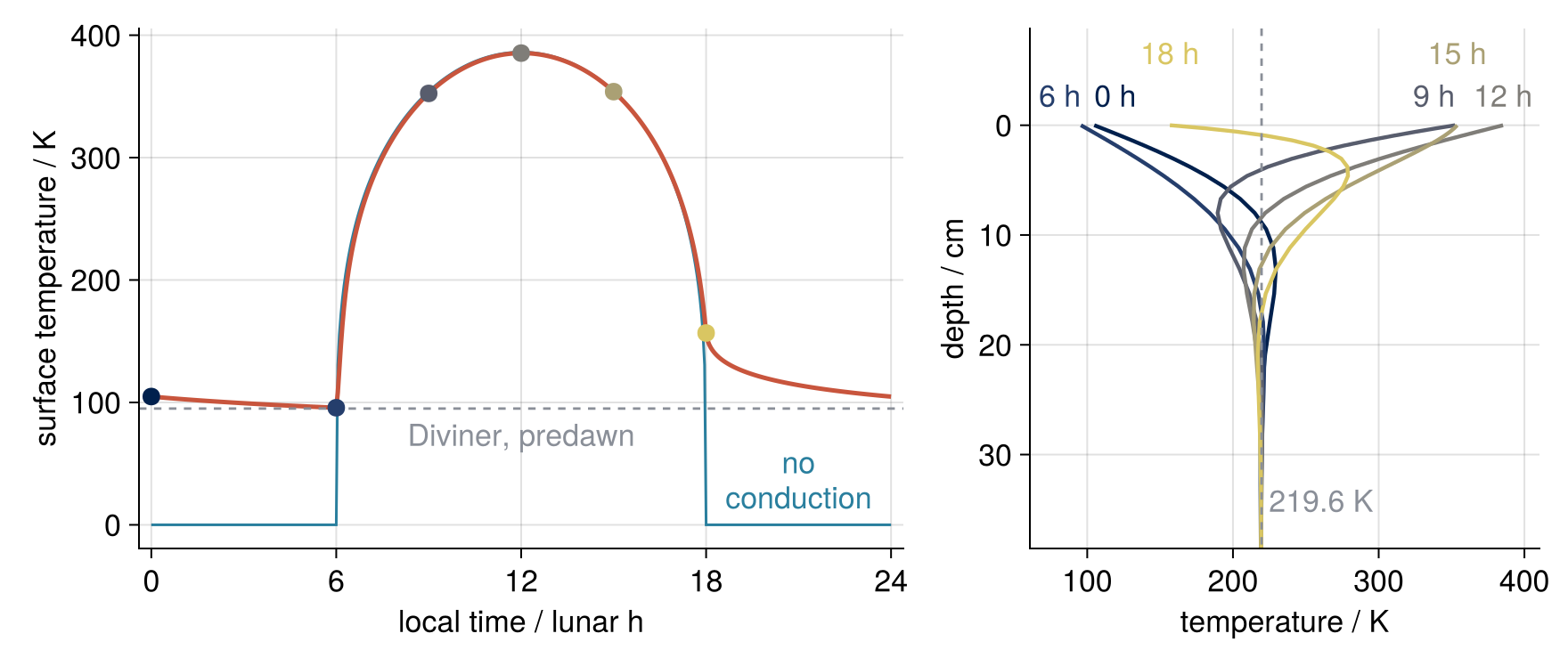
Left: lunar surface temperature in K against local time in lunar hours (one is 29.5 Earth hours). The model stays above the 95 K Diviner line all night, while radiation alone drops to 0 K at sunset. Right: temperature against depth in cm at six times of day; the daily swing dies out within about 30 cm, at 219.6 K.

Trust the surface curve. Its predawn minimum of 95.6 K matches the about 95 K that Diviner measures on the equator, and \(\Gamma = 55\) comes from Hayne et al. (2017), not from a fit: \(\Gamma = 30\) would give 82.8 K, \(\Gamma = 80\) 104.4 K. When the Sun sets, heat stored in the ground still keeps the surface at 156.7 K; radiation alone has already dropped it to 0 K.

The deep temperature is another matter. The probes that Apollo 15 and 17 drilled into the regolith read about 250 K at 1 m, 30 K above the model's 219.6 K, and they sat at 26°N and 20°N, so the gap on the equator is wider still. Constant properties tie the deep value to the mean surface temperature (Step 5), and real regolith does not have them: it conducts better when hot, because heat also crosses the gaps between grains as radiation, and it is more compact below a few centimeters. Adjusting \(\Gamma\) until both numbers fit would hide where the constant-property model stops working; the last variation goes after part of the difference.

Pitfalls

Two days that agree and a deep temperature that is still wrong. Take the shift out, T = sol.u[end], and start again from 250 K. After 35 lunar days two successive surface curves agree within 0.01 K and the loop ends, the surface a mere 0.4 K off before dawn, yet the bottom is stuck at 236.8 K, 17.2 K above the periodic value. Settling takes the column about 105 lunar days, and the daily change at the surface drops below the stop test long before. Keep the shift, and check the bottom of any spin-up against the day-mean surface temperature.

A uniform grid. Place 32 nodes at equal distances and each cell is 3.2 cm, over half of \(\delta\). The predawn minimum is off by just 0.5 K, so the grid seems to pass. Sunrise is where it fails: a thick top layer heats up slowly, and by 6.2 h the surface lags the fine-grid answer by 29.9 K. Even spacing at the 2.75 mm of the geometric top cell takes 364 nodes, twelve times the 30 of Step 2. Judge a grid by the whole curve, never by one number.

Not naming the stiff method. The column is stiff, and a solve call that does not say so pays for it. Drop FBDF() from Step 4 and the suite picks an algorithm that switches between explicit and implicit methods as it goes (sol.alg lists them): 72,898 calls and 1,636 Jacobians for the day, 48 times the calls of FBDF. Pass Tsit5() out of habit and every refinement makes it worse: with the top cell halved it needs 55,503 calls against 1,631 for FBDF, a factor of 34 where Step 4 showed 15, since a thinner top layer settles faster and the explicit steps must follow. Name FBDF(), for the reason of Step 4.

Variations

An asteroid. Since \(\delta\) scales with \(\sqrt{P}\), a 6-hour day on lunar-like regolith gives a skin depth of 5 mm instead of 5.5 cm, and the grid follows. The day length goes into the inputs of Setup; the one change in the code is the bottom, from 1 m to about 20 skin depths (20skin).
Another latitude. For a body with almost no axial tilt, like the Moon, multiply absorbed by \(\cos\varphi\) at latitude \(\varphi\). Apollo 15 landed at \(\varphi\) = 26°.
A finer grid and a cheaper Jacobian. Each layer exchanges heat only with its two neighbors, so the Jacobian is tridiagonal. Pass ODEFunction(rhs!; jac_prototype = Tridiagonal(zeros(n - 1), zeros(n), zeros(n - 1))) from LinearAlgebra to ODEProblem. Layers three apart do not affect each other, so the solver nudges every third layer in one call: 3 calls per Jacobian instead of one per layer, 30 here and hundreds on a fine grid.
Conductivity that grows with temperature. The form of Hayne et al. (2017) is \(k(T) = k_c\,(1 + \chi\,(T/350\ \mathrm{K})^3)\); compute it for each face from the temperatures on both sides, in the flux line of rhs!. Heat then goes down more easily by day than it returns at night, so the deep temperature climbs above the day-mean surface temperature, closing part of the difference of Step 6, and \(\Gamma\) alone no longer sets the curve. The spin-up shift needs a new target too, the \(T_b\) with \(U(T_b) = \langle U(T_0)\rangle\), where \(U(T) = \int k\,dT\); the old one aims too low.

Cheat sheet

skin = sqrt(k / (ρ * c) * P / π)                              # depth of the daily temperature wave
zz = cumsum([0; skin / 20 .* 1.15 .^ (0:59)])                 # top cell skin/20, each next one 15 % thicker
z = [zz[zz .< L]; L]                                          # node depths from the surface to the bottom L
width = diff([0.0; (z[1:end-1] .+ z[2:end]) ./ 2; L])         # each node's layer; half cells at both ends
q = [absorbed(t) - ε * σ * T[1]^4; -k .* diff(T) ./ diff(z); 0.0]   # in rhs!: surface, Fourier's law, closed bottom
dT .= (q[1:end-1] .- q[2:end]) ./ (ρ * c .* width)            # flux in minus flux out; no Float64 buffers
prob = ODEProblem(rhs!, T, (0.0, P), (; z, width, k))
sol = solve(prob, FBDF(); saveat = t, reltol = 1e-6, abstol = 1e-6)   # implicit: the column is stiff
sol.stats.nf, sol.stats.njacs                                 # every call of rhs!, Jacobian calls included
T = sol.u[end] .+ (mean(sol[1, 1:end-1]) - sol.u[end][end])   # spin-up shift; constant k, closed bottom only