The wave equation by leapfrog finite differences in Julia: a pulse on a string

The problem: does a pulse on a string come back as it left?

A string of length L = 1 m is fixed at both ends. Pull up a Gaussian bump of width 3 cm at x = 0.3 m and release it. From then on the displacement \(u(x, t)\) follows the wave equation

\[\frac{\partial^2 u}{\partial t^2} = c^2\,\frac{\partial^2 u}{\partial x^2},\]

for a wave speed c = 1 m/s. Two half-height copies of the bump separate, one heading left and one right; each is turned over by the fixed end it hits, and they meet again.

After 2L/c = 2 s each part of the wave has visited both ends, and the string is back in its initial shape, exactly. That is the yardstick for the leapfrog scheme, written here in Julia: finite differences on a grid stand in for both second derivatives, and each time step is one loop over the grid points. The one number that controls it is the Courant number C = cΔt/Δx: in grid spacings, how far a wave moves per step.

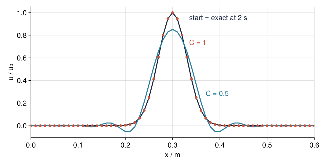
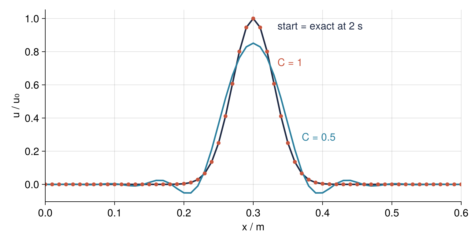
String displacement u / u0 against x in m after a 2 s round trip. C = 1 dots sit on the starting shape; the C = 0.5 curve returns at 0.85 of the height, wider, with dips on both sides.

At C = 1 the string comes home within 2.0 × 10⁻¹⁵, the size of rounding error in double precision. At C = 0.5, after twice as many steps, the peak is down to 85 %, the bump has spread, and a trough sits on either side. Step 6 draws this from earlier runs. Nudge C to 1.01 and nothing survives to be drawn: the error gains about a third at every step and is larger than the pulse itself before the 2 s are up.

Setup

Base Julia handles the arrays and loops, Printf the formatted printing, and CairoMakie the plots. Printf comes with every Julia installation; CairoMakie needs import Pkg; Pkg.add("CairoMakie") once. The four constants describe the string and the bump.

using Printf, CairoMakie

const L = 1.0      # string length, m
const c = 1.0      # wave speed, m/s
const x0 = 0.3     # pulse center, m
const σ = 0.03     # pulse width, m

const INK, ACCENT, SECOND, MUTED = "#1f2a44", "#c8553d", "#2a7f9e", "#8a8f98"
set_theme!(Theme(                          # the look of every figure below
    size = (770, 396), fontsize = 17,
    palette = (color = [INK, ACCENT, SECOND, MUTED],),
    Axis = (topspinevisible = false, rightspinevisible = false, xgridvisible = true, ygridvisible = true),
    Lines = (linewidth = 2.5,),
))

@printf("round trip 2L/c = %.1f s\n", 2L / c)

round trip 2L/c = 2.0 s

Step 1: Put the string on a grid and lay down the pulse

A 1 cm spacing gives 100 intervals and 101 points, ends included. Julia indexes from 1, so the clamp lives in entries 1 and N + 1. pulse takes one position and the dot spreads it over the grid; later steps call it on other grids and at displaced positions:

N = 100
x = collect(range(0, L, length = N + 1))
dx = x[2] - x[1]

pulse(x) = exp(-(x - x0)^2 / (2σ^2))

u0 = pulse.(x)
@printf("dx = %.2f m, %.0f points per σ\n", dx, σ / dx)
@printf("pulse at the ends before clamping: %.1e, %.1e\n", u0[1], u0[end])
u0[[1, end]] .= 0.0;                       # the clamped ends

dx = 0.01 m, 3 points per σ
pulse at the ends before clamping: 1.9e-22, 6.0e-119

Zeroing the ends alters the bump by 1.9 × 10⁻²², invisible to any measurement. Three points per σ is thin on purpose: it just captures the shape, and Step 5 counts the cost.

Step 2: Replace both second derivatives by differences

Add a point's two neighbors, subtract twice the point, divide by the spacing squared, and you have the second derivative to second order. With \(u_j^n\) the value at grid point j after n time steps, call \(\delta^2 u_j = u_{j+1} - 2u_j + u_{j-1}\) this second difference. Doing it once along t and once along x gives

\[\frac{u_j^{n+1} - 2u_j^n + u_j^{n-1}}{\Delta t^2} = c^2\,\frac{\delta^2 u_j^n}{\Delta x^2} \quad\Longrightarrow\quad u_j^{n+1} = 2u_j^n - u_j^{n-1} + C^2\,\delta^2 u_j^n ,\]

after which c, Δt, and Δx appear only through C.

A loop over the interior fills a fresh array of zeros; leaving its end entries alone is the clamp. Julia compiles this loop to machine code. Broadcasting over shifted slices such as u[3:end] would be no faster, since each slice is a fresh copy (Performance Tips, Julia manual). One spike among seven points exposes the weights:

function leapfrog(u, u_old, C2)
    u_new = zero(u)                        # the ends stay at zero: this is the clamp
    for j in 2:length(u)-1
        u_new[j] = 2u[j] - u_old[j] + C2 * (u[j+1] - 2u[j] + u[j-1])
    end
    return u_new
end

spike = zeros(7)
spike[4] = 1.0
for C in [1.0, 0.5]
    println("C = $C: new values at points 3, 4, 5: ", leapfrog(spike, zeros(7), C^2)[3:5])
end

C = 1.0: new values at points 3, 4, 5: [1.0, 0.0, 1.0]
C = 0.5: new values at points 3, 4, 5: [0.25, 1.5, 0.25]

Each neighbor of the spike receives C², and the spike keeps 2 − 2C². When C = 1 the center weight drops out: every new value is its two neighbors summed minus its own old value, so a disturbance advances one point per step, the wave's own speed. In time it leaps from level n − 1 over level n to level n + 1, like one frog vaulting another, which named it.

Step 3: Take the first step from the initial velocity

The update uses two past levels, but at t = 0 you know only the shape and the velocity \(v^0\). Expand in a Taylor series, \(u(\Delta t) = u + \Delta t\,u_t + \tfrac12\Delta t^2 u_{tt}\), and let the wave equation trade \(u_{tt}\) for \(c^2 u_{xx}\):

\[u_j^1 = u_j^0 + \Delta t\, v_j^0 + \tfrac{C^2}{2}\,\delta^2 u_j^0 .\]

Released from rest, the string has \(v^0 = 0\). The check is d'Alembert's solution: two half-size copies of the initial shape, one running each way, \(u = \tfrac12[f(x - ct) + f(x + ct)]\). Away from the walls, \(f\) is the pulse itself:

function first_step(u0, v0, dt, C2)
    u1 = zero(u0)
    for j in 2:length(u0)-1
        u1[j] = u0[j] + dt * v0[j] + 0.5C2 * (u0[j+1] - 2u0[j] + u0[j-1])
    end
    return u1
end

dt = dx / c                                # C = 1
u1 = first_step(u0, zero(x), dt, 1.0)
u1_exact = 0.5 .* (pulse.(x .- c * dt) .+ pulse.(x .+ c * dt))
@printf("largest difference from the exact u at t = dt: %.1e\n", maximum(abs.(u1 .- u1_exact)))

largest difference from the exact u at t = dt: 5.6e-16

With C = 1 the first step averages the shape shifted one point to either side, which is that solution at t = Δt, matched here to 5.6 × 10⁻¹⁶. The first pitfall shows the cost of skipping it with u_old = u0.

Step 4: Run one round trip and check it against the exact solution

Step 3's \(f\) also handles the fixed ends: beyond each end the pulse continues as its own upside-down mirror image, repeating every 2L. Pulse and image cancel at the end, so u there stays zero.

simulate steps the string to t_end and stores level n in column n + 1 of the matrix U. Where t_end / dt is not an integer (C = 0.9 in Step 5), it rounds the step count, adjusts Δt to land on t_end, and returns the C it used. It also returns an energy, a check that needs no exact solution. Divided by the string's mass per length, the energy is

\[E = \frac12\int_0^L \left(u_t^2 + c^2 u_x^2\right)dx .\]

Replace the derivatives by differences at one time level, and the discrete sum varies by 3 % in the exact run below: the differences err, and their error changes whenever the two halves overlap, at the start, the walls, and where they meet. Leapfrog conserves a neighboring sum that takes the velocity between two levels and multiplies the slopes of both, with \(\delta_+ u_j = u_{j+1} - u_j\):

\[E^{n+1/2} = \frac{\Delta x}{2}\sum_j \left[\left(\frac{u_j^{n+1} - u_j^n}{\Delta t}\right)^2 + c^2\,\frac{\delta_+u_j^{n+1}\,\delta_+u_j^n}{\Delta x^2}\right].\]

Multiply Step 2's update by \(u_j^{n+1} - u_j^{n-1}\) and sum over j: velocity and slope terms each collapse into a difference between consecutive steps, and the two cancel.

function exact(x, t)
    function f(s)                          # the pulse, odd about both walls, period 2L
        s = mod(s, 2L)
        return s <= L ? pulse(s) : -pulse(2L - s)
    end
    return 0.5 * (f(x - c * t) + f(x + c * t))
end

function energy(u_new, u, dt, dx)
    kinetic = 0.5 * sum(((u_new .- u) ./ dt) .^ 2) * dx
    strain = 0.5 * c^2 * sum(diff(u_new) .* diff(u)) / dx
    return kinetic + strain
end

function simulate(C, N, t_end; v0 = zeros(N + 1))
    x = collect(range(0, L, length = N + 1))
    dx = x[2] - x[1]
    steps = round(Int, t_end / (C * dx / c))
    dt = t_end / steps
    C2 = (c * dt / dx)^2
    u0 = pulse.(x)
    u0[[1, end]] .= 0.0
    U = zeros(N + 1, steps + 1)            # column n + 1 holds time level n
    U[:, 1] = u0
    U[:, 2] = first_step(u0, v0, dt, C2)
    for n in 2:steps
        U[:, n+1] = leapfrog(U[:, n], U[:, n-1], C2)
    end
    E = [energy(U[:, n+1], U[:, n], dt, dx) for n in 1:steps]
    return x, collect(dt .* (0:steps)), U, sqrt(C2), E
end

x, t, U, C, E = simulate(1.0, 100, 2.0)
for t_check in [0.5, 2.0]
    n = round(Int, t_check / t[2]) + 1
    @printf("t = %.1f s: largest deviation from exact %.1e\n", t[n], maximum(abs.(U[:, n] .- exact.(x, t[n]))))
end
@printf("relative energy drift over the round trip: %.1e\n", (maximum(E) - minimum(E)) / E[1])

t = 0.5 s: largest deviation from exact 1.6e-15
t = 2.0 s: largest deviation from exact 2.0e-15
relative energy drift over the round trip: 5.1e-16

Deviations and drift are rounding noise: at C = 1 the grid values are exact. Earlier levels are drawn lighter:

fig = Figure()
ax = Axis(fig[1, 1], xlabel = "x / m", ylabel = "u / u₀", limits = (nothing, (-1.15, 1.15)), xticks = 0:0.2:1)
for (t_snap, α, (x_lab, y_lab)) in zip([0, 0.25, 0.5, 1.0], [0.3, 0.5, 0.75, 1.0],
                                      [(0.345, 0.85), (0.58, 0.5), (0.83, 0.45), (0.73, -0.95)])
    n = round(Int, t_snap / t[2]) + 1
    lines!(ax, x, U[:, n], color = (ACCENT, α))
    text!(ax, x_lab, y_lab, text = @sprintf("t = %g s", t_snap), color = (ACCENT, 0.55 + 0.45α))   # labels stay legible
end
vlines!(ax, [0, L], color = MUTED, linewidth = 1.2, linestyle = :dash)
fig

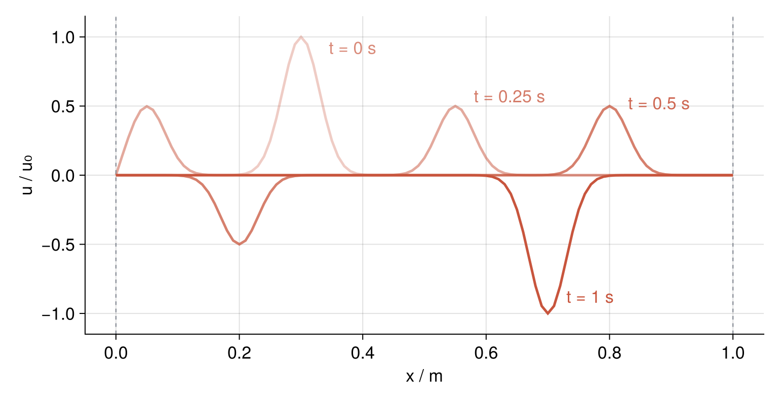
String displacement u / u0 against x in m at t = 0, 0.25, 0.5, and 1 s, leapfrog at C = 1. The pulse splits into two halves, the left half flips at the clamped end x = 0, and at t = 1 s an inverted pulse sits at x = 0.7 m.

By t = 1 s each half has flipped at its own end, and the two overlap at x = 0.7 m as one upside-down pulse.

Step 5: Lower the Courant number and watch the pulse fall apart

With an ODE solver such as DifferentialEquations.jl, smaller steps mean more accuracy. Not here:

runs = Dict()
for C_try in [0.5, 0.9]
    x, t, U, C, E = simulate(C_try, 100, 2.0)
    runs[C_try] = (x, U[:, end])
    @printf("C = %.4f, %d steps: peak %.3f, lowest %.3f, deviation %.3f, energy drift %.0e\n",
            C, length(t) - 1, maximum(U[:, end]), minimum(U[:, end]),
            maximum(abs.(U[:, end] .- exact.(x, t[end]))), (maximum(E) - minimum(E)) / E[1])
end

C = 0.5000, 400 steps: peak 0.851, lowest -0.052, deviation 0.149, energy drift 3e-15
C = 0.9009, 222 steps: peak 0.976, lowest -0.000, deviation 0.024, energy drift 1e-15

At C = 0.5 the peak returns at 0.851, troughs reach −0.052, and the largest error is 0.149. C = 0.9 still errs by 0.024, 10¹³ times more than C = 1. The culprit is numerical dispersion. Put one Fourier mode, \(u_j^n = e^{i(kj\Delta x - \omega n\Delta t)}\), into Step 2's update. The second difference along t multiplies the mode by \(-4\sin^2(\omega\Delta t/2)\), the one along x by \(-4\sin^2(k\Delta x/2)\), so the update holds only if

\[\sin^2\frac{\omega\Delta t}{2} = C^2\sin^2\frac{k\Delta x}{2}, \quad\text{that is,}\quad \sin\frac{\omega\Delta t}{2} = C\,\sin\frac{k\Delta x}{2} .\]

At C = 1 that is ω = ck for all wavelengths. With C < 1 waves travel at ω/k < c, short ones slowest. With Δt = CΔx/c, their speed over c is ωΔt/(C kΔx):

function speed_ratio(C, points_per_wavelength)
    k_dx = 2π / points_per_wavelength
    return 2asin(C * sin(k_dx / 2)) / (C * k_dx)
end

println("points per wavelength:   16      8      6      4")
for C in [1.0, 0.9, 0.5]
    println("C = $C:          ", join([@sprintf("%.3f", speed_ratio(C, p)) for p in [16, 8, 6, 4]], "  "))
end

points per wavelength:   16      8      6      4
C = 1.0:          1.000  1.000  1.000  1.000
C = 0.9:          0.999  0.995  0.991  0.976
C = 0.5:          0.995  0.981  0.965  0.920

The pulse is not a single wave. Its Gaussian spectrum drops off like \(e^{-k^2\sigma^2/2}\), leaving under 1 % of it in wavelengths below about 2σ. With three points per σ, the shortest wavelength that still counts spans six points, where the table gives C = 0.5 a lag of 3.5 %. For your own problems: eight points or more on the shortest wavelength that matters, where the lag is 0.5 % at C = 0.9 and 1.9 % at C = 0.5. Refine at C = 0.5:

ratio(old, new) = isnan(old) ? "       " : @sprintf("(÷%4.1f)", old / new)   # gain over the coarser grid
previous = (NaN, NaN)
for N in [50, 100, 200, 400]
    x, t, U, C, E = simulate(0.5, N, 2.0)
    n_half = round(Int, 0.5 / t[2]) + 1
    dev = (maximum(abs.(U[:, n_half] .- exact.(x, t[n_half]))), maximum(abs.(U[:, end] .- exact.(x, t[end]))))
    @printf("N = %3d: %4.1f points per σ, deviation at 0.5 s %.4f %s, at 2 s %.4f %s, energy drift %.0e\n",
            N, σ * N / L, dev[1], ratio(previous[1], dev[1]), dev[2], ratio(previous[2], dev[2]),
            (maximum(E) - minimum(E)) / E[1])
    global previous = dev
end

N =  50:  1.5 points per σ, deviation at 0.5 s 0.1394        , at 2 s 0.3831        , energy drift 1e-15
N = 100:  3.0 points per σ, deviation at 0.5 s 0.0413 (÷ 3.4), at 2 s 0.1487 (÷ 2.6), energy drift 3e-15
N = 200:  6.0 points per σ, deviation at 0.5 s 0.0101 (÷ 4.1), at 2 s 0.0216 (÷ 6.9), energy drift 5e-15
N = 400: 12.0 points per σ, deviation at 0.5 s 0.0025 (÷ 4.0), at 2 s 0.0016 (÷13.9), energy drift 1e-14

The 0.5 s error drops fourfold with each of the last two halvings: second order. At 2 s the final halving divides it by 13.9, near 16, because a round trip is a full period: every wave returns as cos(2π + ε) ≈ 1 − ε²/2, and with ε ∝ Δx² the error goes as Δx⁴. The energy drift stays under 10⁻¹⁴: no energy disappears, it is handed to short waves trailing the pulse. A finer grid fixes it, a lower C never will.

Step 6: Cross the Courant limit and draw the round trip

Go slightly above C = 1. The shortest wave this grid can hold has two points per wavelength, kΔx = π, and the relation of Step 5 would need sin(ωΔt/2) = C, more than 1, which no real ω gives. Setting ωΔt/2 = π/2 + iy turns the sine into cosh y = C. Where a stable wave only turns its phase, each step now multiplies this one by

\[e^{-i\omega\Delta t} = -e^{2y} = -\left(C + \sqrt{C^2 - 1}\right)^2 = -\left(2C^2 - 1 + 2C\sqrt{C^2 - 1}\right):\]

it flips sign and grows.

The cell takes 200 steps, estimates the amplification per step as the tenth root of the ten-step error ratio, and prints the sign pattern around x = 0.3 m at step 150, since a two-point wave changes sign at every point. t' is a row vector, so exact.(x, t') broadcasts into a matrix with one column per level; maximum with dims = 1 picks the largest entry of each column, and vec flattens the one-row result:

x, t, U, C, E = simulate(1.01, 100, 200 * 1.01 * dx / c)
err = vec(maximum(abs.(U .- exact.(x, t')), dims = 1))
for n in 110:10:200
    @printf("step %d: deviation %8.1e, growth per step %.2f\n", n, err[n+1], (err[n+1] / err[n-9])^0.1)
end
@printf("error above 1 %% from step %d, above the pulse height from step %d\n",
        findfirst(>(0.01), err) - 1, findfirst(>(1), err) - 1)
println("signs at x = 0.25 to 0.35 m, step 150: ", Int.(sign.(U[26:36, 151])))
@printf("growth of the shortest grid wave: %.3f\n", 2C^2 - 1 + 2C * sqrt(C^2 - 1))

step 110: deviation  2.5e-03, growth per step 0.98
step 120: deviation  2.8e-03, growth per step 1.01
step 130: deviation  1.4e-02, growth per step 1.18
step 140: deviation  2.2e-01, growth per step 1.32
step 150: deviation  3.5e+00, growth per step 1.32
step 160: deviation  5.5e+01, growth per step 1.32
step 170: deviation  8.7e+02, growth per step 1.32
step 180: deviation  1.4e+04, growth per step 1.32
step 190: deviation  2.2e+05, growth per step 1.32
step 200: deviation  3.5e+06, growth per step 1.32
error above 1 % from step 129, above the pulse height from step 146
signs at x = 0.25 to 0.35 m, step 150: [-1, 1, -1, 1, -1, 1, -1, 1, -1, 1, -1]
growth of the shortest grid wave: 1.327

fig = Figure(size = (770, 374))
ax = Axis(fig[1, 1], xlabel = "step", ylabel = "largest error / u₀", yscale = log10,
          limits = (0, 200, 1e-5, 1e8),
          yticks = ([1e-4, 1, 1e4, 1e8], ["10⁻⁴", "1", "10⁴", "10⁸"]))
lines!(ax, 1:length(t)-1, err[2:end], color = SECOND)
hlines!(ax, [1], color = MUTED, linewidth = 1.2, linestyle = :dash)
text!(ax, 5, 3, text = "pulse height", color = MUTED)
text!(ax, 166, 1e4, text = "C = 1.01", color = SECOND, align = (:right, :bottom))
fig

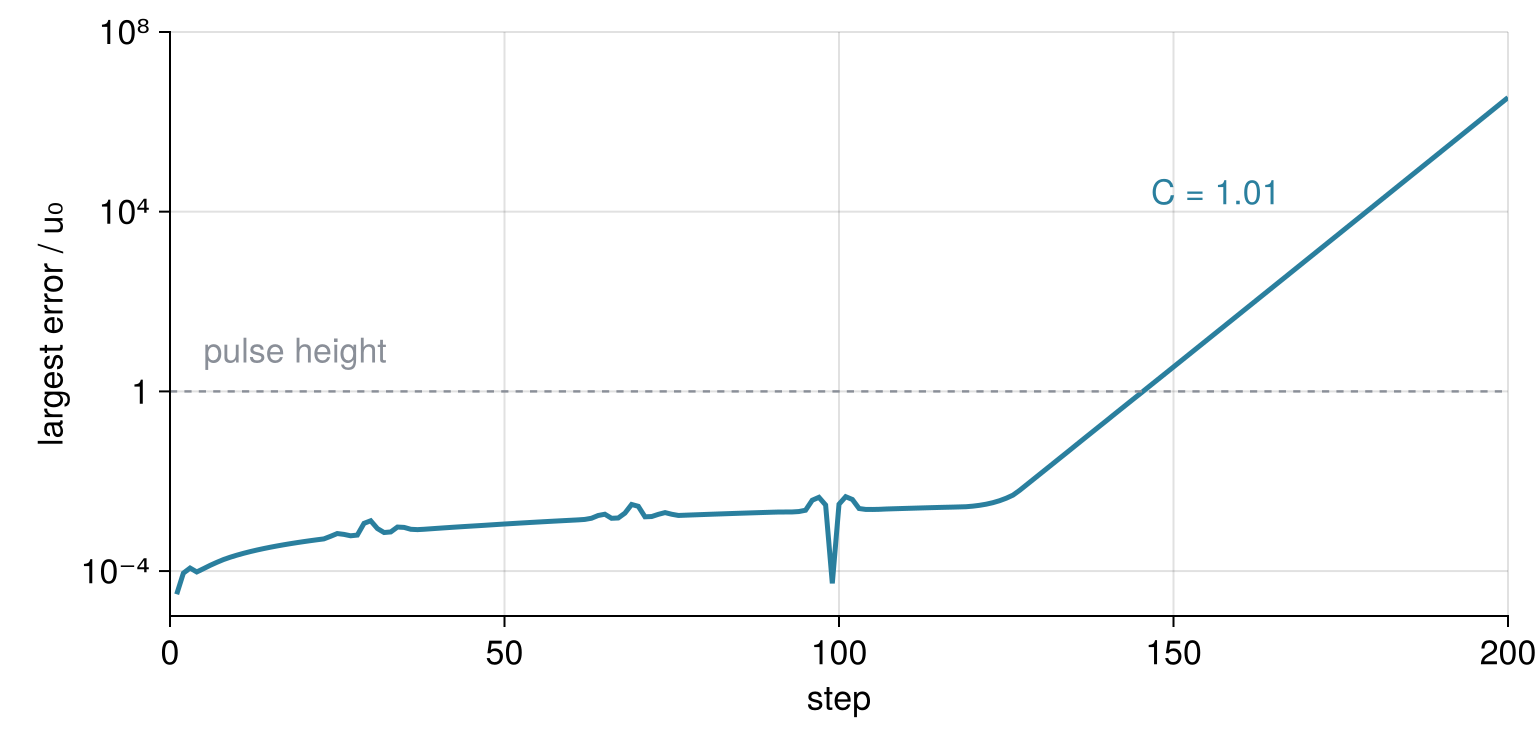
Largest error relative to the pulse height against step number, log scale, for C = 1.01. The error stays below 10⁻² through step 128, then rises on a straight line and crosses the dashed pulse-height level at step 146.

Up to step 128 the error stays within 1 % of the pulse height. After that it rises along a straight line, which on a log axis is a fixed factor per step: 1.32 measured, 1.327 from the formula. From step 146 it exceeds the pulse. The alternating signs identify the two-point wave.

The Gaussian holds none of that wave; rounding errors put it there (see Floating-point numbers, in Python). The same single-wave test gives the stability limit of any explicit linear scheme with constant coefficients.

The figure from the motivation:

x1, t1, U1, _, _ = simulate(1.0, 100, 2.0)
x5, u5 = runs[0.5]
fig = Figure()
ax = Axis(fig[1, 1], xlabel = "x / m", ylabel = "u / u₀", limits = ((0, 0.6), nothing),
          xticks = 0:0.1:0.6, yticks = 0:0.2:1)
lines!(ax, x1, U1[:, 1], color = INK)
lines!(ax, x5, u5, color = SECOND)
scatter!(ax, x1, U1[:, end], color = ACCENT, markersize = 9)
text!(ax, 0.335, 0.92, text = "start = exact at 2 s", color = INK)
text!(ax, 0.335, 0.70, text = "C = 1", color = ACCENT)
text!(ax, 0.37, 0.25, text = "C = 0.5", color = SECOND)
fig

String displacement u / u0 against x in m after a 2 s round trip. C = 1 dots sit on the starting shape; the C = 0.5 curve returns at 0.85 of the height, wider, with dips on both sides.

Pitfalls

Starting with the shape twice. It is tempting to set u_old = copy(u0) and start stepping, and at C = 1 this even survives the round-trip test. Look between periods, though:

for N in [100, 200, 400]
    x = collect(range(0, L, length = N + 1))
    dt = (x[2] - x[1]) / c                 # C = 1
    u = pulse.(x)
    u[[1, end]] .= 0.0
    u_old = copy(u)                        # the shortcut instead of first_step
    levels = [u]
    for n in 1:round(Int, 2.0 / dt)
        u, u_old = leapfrog(u, u_old, 1.0), u
        push!(levels, u)
    end
    n_half = round(Int, 0.5 / dt) + 1
    @printf("N = %d: deviation at t = 0.5 s %.1e, at t = 2 s %.1e\n", N,
            maximum(abs.(levels[n_half] .- exact.(x, 0.5))), maximum(abs.(levels[end] .- exact.(x, 2.0))))
end

N = 100: deviation at t = 0.5 s 5.2e-02, at t = 2 s 1.9e-15
N = 200: deviation at t = 0.5 s 2.5e-02, at t = 2 s 2.6e-15
N = 400: deviation at t = 0.5 s 1.3e-02, at t = 2 s 7.0e-15

Half a second in, the error is 5 % of the pulse height, and it only halves when Δx halves, which makes it first order: this start leaves out the curvature term of Step 3. At 2 s nothing of it remains. With C = 1 all grid waves move at precisely c (Step 5), so after 2L/c the computed string repeats itself for any pair of starting levels, and a round trip returns whatever start it was given. Check at a time between periods, 0.5 s in Step 4, and begin with the first step of Step 3.

Taking dispersion for physics. Wiggles behind a pulse can pass for a stiff string or a dispersive material, and in a synthetic seismogram for the long train of oscillations behind a real arrival (the coda). The test is to halve Δx at the same C. Ripples made by the grid shrink fourfold or more (Step 5); ripples made by the physics do not change.

A time step that was fine on the old grid. Doubling the grid from N = 100 to 200 while keeping Δt = 0.01 s quietly raises C to 2, and by step 16 the alternating wave of Step 6 exceeds 10. Taking Δt from an average speed on a two-material string, or in layered rock, fails the same way, because the fastest c decides. Whenever C, Δx, or the largest c changes, compute Δt again from all three. Waves get off lightly at that. For heat diffusion with an explicit scheme, as in py-pde from the ground up (in Python), Δt must fall with Δx², so every halving of the grid multiplies the number of steps by four.

Variations

One-way pulse. Give simulate the keyword v0 = -c .* dpulse.(x), dpulse being the derivative of the pulse, and the bump moves right as a whole instead of splitting; first_step needs no change.
A free end. At x = L, drop the clamp and add a ghost point beyond the last one that mirrors the point before it, \(u_{N+2} = u_N\) with Julia's indices. That sets ∂u/∂x = 0 and lets the loop include j = N + 1. Reflection there keeps the pulse upright, so it reappears in its starting shape after 4L/c = 4 s, two round trips.
A string of two materials. Turn c into a vector, give C2 a value at every point, and take the limit from the highest c. At the junction, part of the pulse bounces back, like a seismic wave meeting a layer boundary.
A membrane. Two dimensions, the same update with the five-point Laplacian. Stability now needs C ≤ 1/√2, and no choice of C removes dispersion in all directions.

Cheat sheet

x = collect(range(0, L, length = N + 1)); dx = x[2] - x[1]
dt = C * dx / c_max                        # C ≤ 1, with the largest wave speed
C2 = (c * dt / dx)^2
u_old, u = u0, first_step(u0, v0, dt, C2)  # u0 + dt v0 + C2/2 δ²u0, never u_old = u0
for j in 2:N                               # interior points; the compiled loop is fast
    u_new[j] = 2u[j] - u_old[j] + C2 * (u[j+1] - 2u[j] + u[j-1])
end
u_new[1] = u_new[end] = 0.0                # clamped ends
E = 0.5sum(((u_new .- u) ./ dt) .^ 2) * dx + 0.5c^2 * sum(diff(u_new) .* diff(u)) / dx
# C = 1 is exact in 1D with constant c; below 1, more points per wavelength against dispersion