The standard error of the mean in Julia: four times the data, half the error

The question

Twelve batches of a synthesis come off the bench, and you weigh the product of each. Their yields average 49.34 mg. Two more numbers usually travel with that average as error bars: the standard deviation, 2.31 mg, and the standard error of the mean, 0.67 mg. A colleague then makes 36 batches more. The upper row shows the first twelve, the lower row all 48:

Show code

using CairoMakie, Statistics, StatsBase, Distributions, Random, Printf

const INK, ACCENT, SECOND, MUTED = "#1f2a44", "#c8553d", "#2a7f9e", "#8a8f98"
set_theme!(Theme(
    size = (770, 352), fontsize = 17,
    palette = (color = [INK, ACCENT, SECOND, MUTED],),
    Axis = (topspinevisible = false, rightspinevisible = false, xgridvisible = true, ygridvisible = true),
    Lines = (linewidth = 2.5,),
))

# The batches are simulated from a known truth and rounded like a balance reading.
const MU, SIGMA = 50.0, 2.5                                    # mg
twelve = round.(rand(Xoshiro(1968), Normal(MU, SIGMA), 12), digits = 1)
more = round.(rand(Xoshiro(27), Normal(MU, SIGMA), 36), digits = 1)
batches48 = [twelve; more]

for x in (twelve, batches48)
    @printf("%2d batches: mean %6.2f mg   sd %4.2f mg   standard error %4.2f mg\n",
            length(x), mean(x), std(x), sem(x))
end

fig = Figure()
ax = Axis(fig[1, 1], xlabel = "yield / mg", ygridvisible = false,
          yticks = ([0.35, 1.35], ["48 batches", "12 batches"]))
offsets = repeat([0.30, 0.42, 0.54, 0.36, 0.48, 0.60], 8)     # fixed heights, so dots do not hide each other
for (row, x) in zip((1, 0), (twelve, batches48))
    m, sd, se = mean(x), std(x), sem(x)
    scatter!(ax, x, row .+ offsets[1:length(x)], color = INK, markersize = 8)
    linesegments!(ax, [m - sd, m + sd], fill(row + 0.12, 2), color = SECOND, linewidth = 2, linecap = :butt)
    linesegments!(ax, [m - se, m + se], fill(row + 0.02, 2), color = ACCENT, linewidth = 6, linecap = :butt)
    text!(ax, m + sd + 0.2, row + 0.12, text = @sprintf("sd %.2f mg", sd), color = SECOND, align = (:left, :center))
    text!(ax, m + sd + 0.2, row + 0.0, text = @sprintf("standard error %.2f mg", se), color = ACCENT,
          align = (:left, :center))
end
xlims!(ax, 43.5, 58.5); ylims!(ax, -0.15, 1.8)
fig

12 batches: mean  49.34 mg   sd 2.31 mg   standard error 0.67 mg
48 batches: mean  50.16 mg   sd 2.30 mg   standard error 0.33 mg

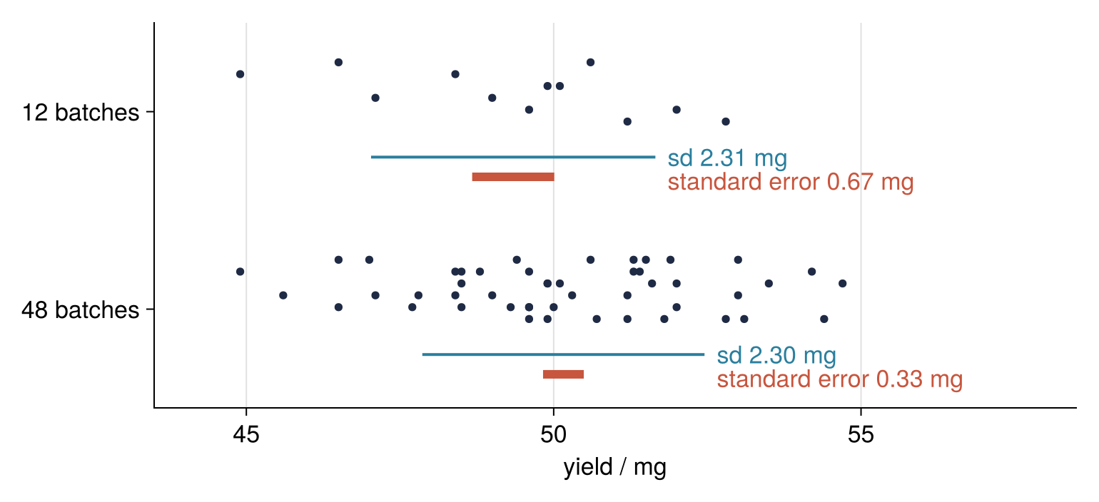
Yields of 12 and of 48 weighed batches, in mg, as dots. The standard-deviation bars are the same width, 2.31 and 2.30 mg; the standard-error bar halves, from 0.67 to 0.33 mg.

Some of this is no surprise. The 48 dots spread over the same range as the twelve, and the standard deviation hardly changes, 2.31 mg against 2.30 mg. Extra batches do not make any single batch more reproducible.

The standard error behaves differently. It went from 0.67 to 0.33 mg: four times the data, half the error, where a quarter would seem natural. The standard deviation belongs to the batches, the standard error to their mean. What is the standard error a measure of, and why does quadrupling the data cut it in half?

I simulated the batches from a truth I set myself, mean μ = 50.0 mg and standard deviation σ = 2.5 mg, and rounded each yield to 0.1 mg like a balance display. The 2.31 mg is therefore not σ but an estimate of it from twelve values; call it s. Julia's std divides by n − 1, not n (corrected = true): twelve values lie slightly closer to their own mean than to μ, and the smaller divisor compensates. The batches stand in for anything you measure repeatedly and average, replicate wells for instance.

A random number generator started from a fixed number, its seed, repeats the same draws on every run. The first twelve yields come from the seed of protocol A in HypothesisTests.jl from the ground up. For the other 36 I tried seeds from 1 upward and kept 27, the first whose 48 yields keep the standard deviation steady and halve the standard error to two decimals; most data sets halve it only roughly. The simulations below use a generator of their own, so no conclusion rests on that choice.

The idea: rerun the experiment and watch the means

Your experiment of twelve batches produced one mean, 49.34 mg. Do the whole thing again with twelve new batches and you get a different mean, and a third run gives a third. Over many runs these means pile up around 50 mg, in a tighter cluster than the single batches form. That cluster's standard deviation is what the standard error of the mean measures: how much the mean would wobble if you could redo the entire experiment again and again. In reality you get one run, so it estimates the wobble from its own data as s/√n.

The cluster is tighter because batches above 50 mg and batches below it offset each other inside one experiment. A lone batch is more than 1 mg off quite often. A mean of twelve is that far off only when most of its batches err the same way, which becomes unlikely fast as n grows. Since I know the truth, the computer can perform the experiment 10,000 times and simply count. The function experiments(n) returns a matrix with one experiment per row, mean(X; dims = 2) takes the mean of each row, and vec flattens the result into an ordinary vector. The mean of a vector of true and false values is the share of trues, which gives the counts:

sim = Xoshiro(2026)

"R repeated experiments of n batches each, drawn from the truth: an R × n matrix in mg."
experiments(n; R = 10_000) = rand(sim, Normal(MU, SIGMA), R, n)

for n in (1, 12, 48)
    means = vec(mean(experiments(n); dims = 2))
    off = mean(abs.(means .- MU) .> 1.0)
    @printf("n = %2d: %4.1f %% of %d means miss 50 mg by more than 1 mg\n", n, 100off, length(means))
end

n =  1: 68.9 % of 10000 means miss 50 mg by more than 1 mg
n = 12: 17.2 % of 10000 means miss 50 mg by more than 1 mg
n = 48:  0.5 % of 10000 means miss 50 mg by more than 1 mg

For single batches the miss rate is 68.9 %, roughly seven in ten. Means of twelve miss in 17.2 % of the runs, one in six, and means of 48 in 0.5 %, one in two hundred. Offsetting errors alone account for all of that.

The histograms below give a width of 0.72 mg for twelve batches, not the 0.67 mg from the opening. Both numbers divide a standard deviation by √12, a factor the Formalization explains. The simulation knows σ, so its means of twelve have a standard deviation of 2.5/√12 = 0.72 mg. The twelve batches of the opening know only their s and put the same quantity at 2.31/√12 = 0.67 mg. One is the true value, the other what a single experiment can make of it.

Ten thousand simulated means for each of three experiment sizes, each histogram on top of the distribution of single batches:

Show code

x_grid = range(43, 57, length = 400)
batch_curve = pdf.(Normal(MU, SIGMA), x_grid)

fig = Figure(size = (770, 693))
axes = [Axis(fig[i, 1], yticksvisible = false, yticklabelsvisible = false) for i in 1:3]
for (ax, n) in zip(axes, (3, 12, 48))
    means = vec(mean(experiments(n); dims = 2))
    hist!(ax, means, bins = 43:0.2:57, normalization = :pdf, color = (ACCENT, 0.6))   # area 1, like the curve
    lines!(ax, x_grid, batch_curve, color = INK)
    vlines!(ax, [MU], color = MUTED, linewidth = 1.4, linestyle = :dash)
    text!(ax, 0.99, 0.92, text = @sprintf("n = %d, sd of means %.2f mg", n, std(means)),
          space = :relative, align = (:right, :top), color = ACCENT)
end
linkxaxes!(axes...); linkyaxes!(axes...)                       # one y scale: the curve stays put
hidexdecorations!.(axes[1:2], grid = false)
axes[2].ylabel = "share per mg"
axes[3].xlabel = "yield / mg"
text!(axes[1], 43.1, 0.07, text = "single batches", color = INK, align = (:left, :bottom))   # above the left tail
xlims!(axes[3], 43, 57); ylims!(axes[3], 0, nothing)
fig

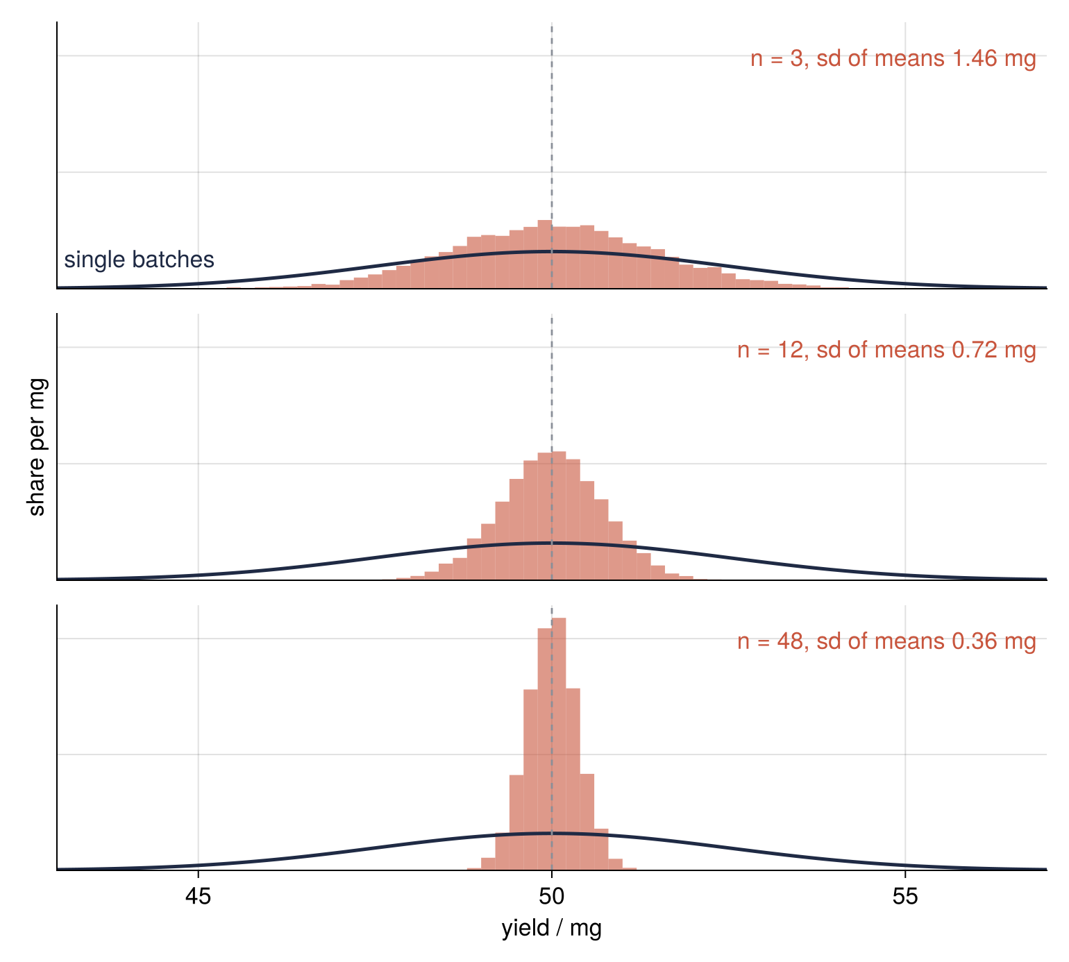
Histograms of 10,000 simulated means of 3, 12, and 48 batches, yield in mg, over the curve of single batches, drawn at the same scale in every panel; dashed line at the true 50 mg. The sd of the means falls from 1.46 to 0.72 to 0.36 mg: each fourfold n halves the width.

Each histogram has an area of 1, like the batch curve, so both fit on one axis, and all three panels share their vertical scale: a histogram half as narrow must rise twice as high. The dashed line marks μ = 50 mg. Going from 3 batches to 12 cuts the width of the means from 1.46 to 0.72 mg, and going from 12 to 48 cuts it to 0.36 mg. The batch curve is identical in all three panels.

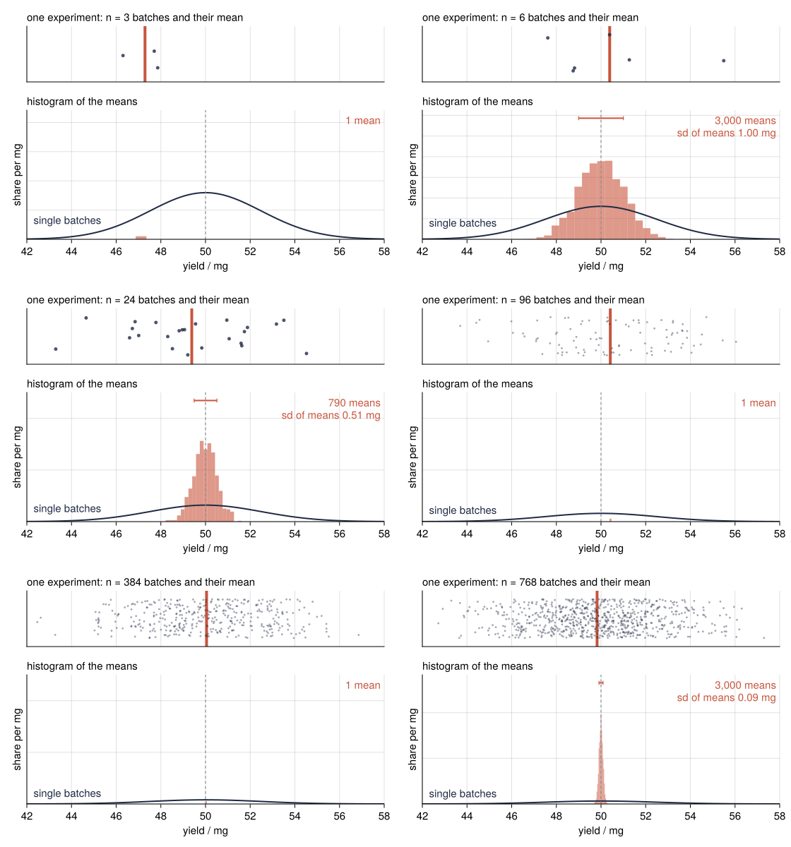
In the animation the histogram grows one experiment at a time:

Animation: experiments of n batches are drawn one after another, and their means pile up into a histogram over the curve of single batches. Each time n doubles the histogram narrows; every two doublings its width halves.

Show code

# Means narrowing: repeated experiments of n batches, and the histogram of their means.
# Each frame draws more experiments of n batches from the truth of the tutorial
# (50.0 mg, sd 2.5 mg), shows the latest one, and adds the means to the histogram
# below; n doubles from 3 to 768. Run from this directory, in the repository's project:
#
#     JULIA_PROJECT=../../../../.. julia scene.jl
#
# Writes ../../assets/means-narrowing.gif.
using CairoMakie, Distributions, Random, Statistics, Printf

const INK, ACCENT, MUTED = "#1f2a44", "#c8553d", "#8a8f98"
const OUT = joinpath(@__DIR__, "..", "..", "assets", "means-narrowing.gif")

# ---- data: R experiments for each n, drawn once from the truth
const MU, SIGMA, R, K0 = 50.0, 2.5, 3000, 200
rng = Xoshiro(2026)
ns = 3 .* 2 .^ (0:8)                                       # 3, 6, ..., 768 batches
runs = Dict(n => rand(rng, Normal(MU, SIGMA), R, n) for n in ns)
heights = Dict(n => rand(rng, n) .* 0.7 .+ 0.15 for n in ns)   # fixed heights for the dots

# ---- frames: (n, number of experiments so far); a longer hold on 12 and 48
frames = Tuple{Int, Int}[]
for n in ns
    len = n in (12, 48) ? 14 : 10
    counts = unique(round.(Int, exp.(range(0, log(R), length = len - 3))))
    append!(frames, [(n, k) for k in [counts; fill(R, len - length(counts))]])
end

# ---- the figure, drawn once; Observables carry what changes
set_theme!(Theme(fontsize = 15, Axis = (topspinevisible = false, rightspinevisible = false,
                                        titlealign = :left, titlefont = :regular)))
fig = Figure(size = (560, 400))
ax1 = Axis(fig[1, 1], yticksvisible = false, yticklabelsvisible = false, ygridvisible = false)
ax2 = Axis(fig[2, 1], title = "histogram of the means", xlabel = "yield / mg", ylabel = "share per mg",
           yticksvisible = false, yticklabelsvisible = false)
rowsize!(fig.layout, 1, Relative(0.3))
linkxaxes!(ax1, ax2); hidexdecorations!(ax1, grid = false)
xlims!(ax2, 42, 58); ylims!(ax1, 0, 1)

state = Observable(frames[1])
n_now = @lift $state[1]
latest = @lift runs[$state[1]][$state[2], :]                # the batches of the latest experiment
means = @lift vec(mean(runs[$state[1]][1:$state[2], :]; dims = 2))
se = @lift SIGMA / sqrt($n_now)

vlines!(ax1, @lift([mean($latest)]), color = ACCENT, linewidth = 4)
scatter!(ax1, latest, @lift(heights[$n_now]), color = @lift(($n_now <= 48 ? (INK, 0.8) : (INK, 0.4))),
         markersize = @lift($n_now <= 48 ? 7 : 4))                # dots above the mean, never hidden by it

# The first K0 means pile up as blocks of equal height; from K0 on the histogram is a density.
# This keeps a few early means from shooting through the top of the panel.
bars = @lift begin
    w = $se / 3
    edges = MU - 5 * $se - w / 2 : w : MU + 5 * $se + w
    counts = [count(e -> lo <= e < lo + w, $means) for lo in edges[1:end-1]]
    Point2f.(edges[1:end-1] .+ w / 2, counts ./ (max(length($means), K0) * w))
end
barplot!(ax2, bars, gap = 0, width = @lift($se / 3), color = (ACCENT, 0.6), strokewidth = 0)
x_grid = range(42, 58, length = 400)
lines!(ax2, x_grid, pdf.(Normal(MU, SIGMA), x_grid), color = INK, linewidth = 2)
vlines!(ax2, [MU], color = MUTED, linewidth = 1.2, linestyle = :dash)

peak = @lift 1 / ($se * sqrt(2π))
many = @lift length($means) > 1                             # one mean has no spread to show
sd_now = @lift $many ? std($means) : 0.0
bracket = @lift [Point2f(MU - $sd_now, 1.5 * $peak), Point2f(MU + $sd_now, 1.5 * $peak)]
lines!(ax2, bracket, color = ACCENT, linewidth = 2, visible = many)   # ± one sd of the means, with end caps
scatter!(ax2, bracket, marker = :vline, markersize = 9, color = ACCENT, visible = many)
# Name the batch curve on its left flank, lifted above the curve 3.2 mg further right, so the
# label clears it however tall the y axis grows.
label_y = @lift pdf(Normal(MU, SIGMA), 42.3 + 3.2) + 0.03 * 1.6 * $peak
text!(ax2, @lift(Point2f(42.3, $label_y)), text = "single batches", color = INK, align = (:left, :bottom))
thousands(k) = replace(string(k), r"(?<=\d)(?=(\d{3})+$)" => ",")   # 3000 -> "3,000"
label = @lift $many ? @sprintf("%s means\nsd of means %.2f mg", thousands(length($means)), $sd_now) : "1 mean"
text!(ax2, 0.99, 0.97, text = label, space = :relative, align = (:right, :top), color = ACCENT)
on(peak) do p                                               # the y axis follows the narrowing histogram
    ylims!(ax2, 0, 1.6 * p)
end
ylims!(ax2, 0, 1.6 * peak[])

record(fig, OUT, frames; framerate = 12, px_per_unit = 1) do f
    state[] = f
    ax1.title = "one experiment: n = $(f[1]) batches and their mean"
end
@printf("wrote %s: %d frames, %d kB\n", OUT, length(frames), filesize(OUT) ÷ 1024)

The upper panel holds the batches of the current experiment as dots, with their mean as a vertical line. The first means fall all over the place, and only after some hundreds does the histogram look like a curve. Then n doubles, the count restarts, and the new histogram comes out narrower, while the dots above remain as scattered as before. Two doublings of n buy one halving of the width: the means narrow as 1/√n, not as 1/n.

Formalization

The variance is the square of the standard deviation, the mean squared distance from the mean: σ = 2.5 mg becomes 6.25 mg². The derivation uses variances because two rules hold for them that fail for standard deviations.

Rule 1: for independent values, variances add. When one value carries no information about the other, \(\operatorname{Var}(X_1 + X_2) = \operatorname{Var}(X_1) + \operatorname{Var}(X_2)\).

Rule 2: multiply a value by c, and its variance is multiplied by c². Halve each value and the variance drops to a quarter: \(\operatorname{Var}(cX) = c^2 \operatorname{Var}(X)\).

A test on 100,000 simulated pairs of batches:

pair = vec(sum(rand(sim, Normal(MU, SIGMA), 100_000, 2); dims = 2))   # two independent batches, added
@printf("Var(X1 + X2)       = %6.3f mg²   rule 1: 2 × 6.25 = 12.500 mg²\n", var(pair))
@printf("Var((X1 + X2) / 2) = %6.3f mg²   rule 2: 12.5 / 4 =  3.125 mg²\n", var(pair ./ 2))

Var(X1 + X2)       = 12.483 mg²   rule 1: 2 × 6.25 = 12.500 mg²
Var((X1 + X2) / 2) =  3.121 mg²   rule 2: 12.5 / 4 =  3.125 mg²

The variance of the sum is 12.48 mg² where rule 1 predicts 12.5, and half the sum gives 3.12 mg² where rule 2 predicts 3.125. The gaps are sampling noise.

Apply the rules to the mean of n batches, \(\bar x = (X_1 + \dots + X_n)/n\). Rule 1 gives the sum n times the variance of one batch; dividing by n means c = 1/n, so rule 2 shrinks that by n², and a square root returns to a standard deviation:

\[\operatorname{Var}(X_1 + \dots + X_n) = n\sigma^2, \qquad \operatorname{Var}(\bar x) = \frac{n\sigma^2}{n^2} = \frac{\sigma^2}{n}, \qquad \mathrm{SE} = \frac{\sigma}{\sqrt{n}} ,\]

where σ belongs to a single batch and SE, the standard error of the mean, is 0.72 mg at n = 12.

Picture the square root this way. Treat the error of each batch as a step of random size, forward or backward from μ. Over n steps they partly cancel, and the total typically lands √n step lengths from the start, not n: rule 1 again, since n times the variance is √n times the standard deviation. Such a path is called a random walk. Divide its end point by n and 1/√n is left.

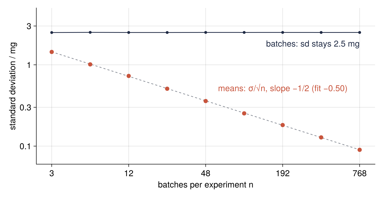
On logarithmic axes a law like this is a straight line. The logarithm of SE = σ/√n is \(\log \mathrm{SE} = \log \sigma - \tfrac{1}{2} \log n\), a line in log n with slope −½, where a 1/n law would have slope −1. The cell runs the simulation from 3 to 768 batches per experiment and measures the slope with a least-squares line through log sd against log n, the regression of a first statistics course, which A \ y with a tall matrix A computes in Julia.

ns = 3 .* 2 .^ (0:8)                                           # 3, 6, 12, ..., 768
sd_means, sd_batches = Float64[], Float64[]
println("   n   sd of the means   σ/√n       sd of the batches")
for n in ns
    X = experiments(n)
    push!(sd_means, std(vec(mean(X; dims = 2))))
    push!(sd_batches, std(X))
    @printf("%4d   %6.3f mg       %6.3f mg   %6.3f mg\n", n, sd_means[end], SIGMA / sqrt(n), sd_batches[end])
end

intercept, slope = [ones(length(ns)) log.(ns)] \ log.(sd_means)
worst = maximum(abs.(sd_means ./ (SIGMA ./ sqrt.(ns)) .- 1))
@printf("fitted slope on log-log axes: %.2f   largest miss against σ/√n: %.1f %%\n", slope, 100worst)

   n   sd of the means   σ/√n       sd of the batches
   3    1.439 mg        1.443 mg    2.493 mg
   6    1.012 mg        1.021 mg    2.506 mg
  12    0.730 mg        0.722 mg    2.497 mg
  24    0.508 mg        0.510 mg    2.496 mg
  48    0.358 mg        0.361 mg    2.501 mg
  96    0.253 mg        0.255 mg    2.500 mg
 192    0.182 mg        0.180 mg    2.501 mg
 384    0.128 mg        0.128 mg    2.499 mg
 768    0.090 mg        0.090 mg    2.499 mg
fitted slope on log-log axes: -0.50   largest miss against σ/√n: 1.1 %

All rows match σ/√n within about 1 %, the largest gap being 0.730 against 0.722 mg at n = 12, and the fitted slope comes out at −0.50, the 1/√n law. The standard deviation of the batches stays between 2.49 and 2.51 mg at every size. More batches pin down the mean, not the batches.

Show code

fig = Figure(size = (770, 396))
ax = Axis(fig[1, 1], xscale = log10, yscale = log10,
          xlabel = "batches per experiment n", ylabel = "standard deviation / mg",
          xticks = (ns[1:2:end], string.(ns[1:2:end])),
          yticks = ([0.1, 0.3, 1, 3], ["0.1", "0.3", "1", "3"]))
scatterlines!(ax, ns, sd_batches, color = INK, markersize = 8)
lines!(ax, ns, SIGMA ./ sqrt.(ns), color = MUTED, linewidth = 1.4, linestyle = :dash)
scatter!(ax, ns, sd_means, color = ACCENT, markersize = 12)
text!(ax, ns[end], 2.1, text = "batches: sd stays 2.5 mg", color = INK, align = (:right, :top))   # under the line, clear of the 3 mg grid line
text!(ax, 60, 0.45, text = replace(@sprintf("means: σ/√n, slope −1/2 (fit %.2f)", slope), "-" => "−"),
      color = ACCENT, align = (:left, :bottom))
ylims!(ax, 0.06, 5)
fig

Log-log plot of standard deviation in mg against batches per experiment, 3 to 768. The sd of the batches stays flat at 2.5 mg; the sd of the means falls on the line σ/√n, fitted slope −0.50.

Three consequences follow.

One tenth the error costs one hundred times the batches. To get from 0.72 mg at twelve batches to 0.072 mg you need 1,200 batches.

In practice σ is estimated. A real experiment reports s/√n, the 0.67 mg of the opening. Means of many independent values follow a normal curve closely, whatever the shape of the single values (the central limit theorem). A normal curve holds 95 % of its values within two standard deviations of its center, and for means of twelve that is 2σ/√12 = 1.44 mg. In 95 % of repeated experiments the mean lands within 1.44 mg of μ, and the interval mean ± 1.44 mg contains μ. Single batches would need ±2σ = ±5 mg, √12 = 3.5 times wider. With s, itself uncertain, in place of σ, the factor 2 becomes 2.20; the next section tests it.

Only independent errors average away. Give all batches of one experiment a common offset, a balance calibration error drawn with a standard deviation of 0.5 mg per experiment, and repeat the sweep. Broadcasting adds each of the 10,000 offsets to every batch in its row:

println("   n   sd of the means   √(0.5² + σ²/n)   without the offset")
for n in ns[1:2:end]
    X = experiments(n) .+ rand(sim, Normal(0, 0.5), 10_000)    # one offset per row, shared by its batches
    @printf("%4d   %6.3f mg       %6.3f mg       %6.3f mg\n",
            n, std(vec(mean(X; dims = 2))), sqrt(0.5^2 + SIGMA^2 / n), SIGMA / sqrt(n))
end

   n   sd of the means   √(0.5² + σ²/n)   without the offset
   3    1.526 mg        1.528 mg        1.443 mg
  12    0.888 mg        0.878 mg        0.722 mg
  48    0.618 mg        0.617 mg        0.361 mg
 192    0.527 mg        0.532 mg        0.180 mg
 768    0.502 mg        0.508 mg        0.090 mg

This time the standard deviation of the means bottoms out at 0.5 mg: 0.50 mg at 768 batches, where the sweep without it gave 0.09 mg. Offset and batch mean are independent, so rule 1 adds their variances, 0.5² + 2.5²/n, of which only the second part falls with n. Rule 1 assumed independence, and a floor is the price of breaking it.

See it in code

Statistics provides mean and std and stops there; the standard error is sem from StatsBase:

Show code

println("              sem          s/√n (by hand)   σ/√n (truth)")
for (name, x) in (("12 batches", twelve), ("48 batches", batches48))
    n = length(x)
    @printf("%-12s  %6.4f mg   %6.4f mg        %6.4f mg\n", name, sem(x), std(x) / sqrt(n), SIGMA / sqrt(n))
end
t95 = quantile(TDist(11), 0.975)
@printf("\nt factor for a 95 %% interval, 12 batches: %.2f\n", t95)

# 10,000 experiments of twelve: how often does mean ± k s/√12 contain the true 50 mg?
X = experiments(12)
half = vec(std(X; dims = 2)) ./ sqrt(12)
for k in (2.0, t95)
    hit = mean(abs.(vec(mean(X; dims = 2)) .- MU) .< k .* half)
    @printf("mean ± %.2f s/√12 contains 50 mg in %4.1f %% of %d experiments\n", k, 100hit, size(X, 1))
end

              sem          s/√n (by hand)   σ/√n (truth)
12 batches    0.6677 mg   0.6677 mg        0.7217 mg
48 batches    0.3313 mg   0.3313 mg        0.3608 mg

t factor for a 95 % interval, 12 batches: 2.20
mean ± 2.00 s/√12 contains 50 mg in 93.3 % of 10000 experiments
mean ± 2.20 s/√12 contains 50 mg in 95.3 % of 10000 experiments

sem and std(x) / sqrt(length(x)) print the same digits, since both use n − 1. In Float64 they may disagree in the final bit, because sem computes the square root of var(x) / n. At both sizes the estimate lies under the truth, 0.67 against 0.72 mg for twelve batches and 0.33 against 0.36 mg for 48: these particular yields scatter slightly less than σ, and s carries that over. A different seed could put either one above.

The factor 2.20 for an interval from s comes from Student's t distribution. Its one parameter is n − 1, here 11, and the fewer values s rests on, the larger the factor. In the simulation the factor 2 catches 50 mg in 93.3 % of experiments, the factor 2.20 in 95.3 %. Step 2 of HypothesisTests.jl from the ground up constructs this interval.

The definition decides which bar belongs in a figure. Draw the standard deviation to show how much individual measurements vary, a gene's expression from cell to cell, say. Draw the standard error to show how precisely you know the average. Name the choice in the caption: a bar looks the same either way.

Where it shows up

Chemistry and biology. Bar charts of triplicates or of three mice in each group carry error bars that are standard deviations in one paper and standard errors in the next, and with n = 3 they differ by a factor √3 = 1.7. Three wells filled from one culture are technical replicates and inherit whatever went wrong in that culture, so only separate cultures or animals, the biological replicates, let that error average out.
Physics and mathematics. A Monte Carlo integral or mean energy is the average of N random samples, its error shrinks as 1/√N whatever the dimension, and so every extra correct digit costs a hundredfold the samples. A poll obeys the same law, where p(1 − p) is the variance of one yes-or-no answer at share p, so asking 1,000 people about a 50 % share gives √(0.5 × 0.5 / 1000), roughly 1.6 percentage points.
Engineering and spectroscopy. Averaging 64 sweeps on an oscilloscope, or adding up 64 scans in an NMR spectrometer, multiplies the signal-to-noise ratio by √64 = 8: the signal is identical in every pass and the noise is not. A doubled signal-to-noise ratio takes four times as long to record.
Geology. Averaging the ages of 20 zircon grains from one rock, weighted by their precision, cuts the random error by √20 = 4.5 compared with one grain. The decay constant and the calibration against a reference standard affect every grain alike and stay as they are; they are the common offset of the third consequence, which geochronologists quote as a separate systematic error.

The rule behind every item: averaging N measurements divides their independent errors by √N and leaves the error they have in common untouched.

The question

The idea: rerun the experiment and watch the means

Formalization

See it in code

Where it shows up

Further reading