Dealiasing: why a product on a grid can blow up a spectral solver (Python)

The question

Start the inviscid Burgers equation, \(u_t + u\,u_x = 0\), from \(u = \sin x\) on the periodic interval \([0, 2\pi)\), and solve it the way the KdV tutorial solves KdV, with derivatives by FFT and the product \(u\,u_x\) formed on the grid, but without its 2/3 mask: 64 grid points and classical RK4 with a step of \(2.5 \times 10^{-4}\). Nothing in it guards against aliasing. At t = 2.258 the run blows up: the energy passes 100 times its starting value.

What should happen is quick to say. Each point of the profile moves at a speed equal to its own height (along its characteristic). The crest at \(x = \pi/2\) runs right at speed 1, the trough at \(3\pi/2\) runs left, and the slope at \(x = \pi\), where the two meet, steepens until it is vertical at \(t = 1/\max|u_0'| = 1\). Past that moment the formula would give three values of \(u\) at one \(x\). The physical solution, the limit of a vanishing viscosity, is a jump standing at \(x = \pi\), and the jump dissipates energy.

Show code

import numpy as np
import matplotlib.pyplot as plt
from numpy.fft import rfft, irfft

plt.rcParams.update({
    "figure.figsize": (7, 4.5), "figure.dpi": 110,
    "axes.spines.top": False, "axes.spines.right": False,
    "axes.grid": True, "grid.alpha": 0.25,
    "font.size": 11, "lines.linewidth": 1.8,
})
INK, ACCENT, SECOND, MUTED = "#1f2a44", "#c8553d", "#2a7f9e", "#8a8f98"

# ---- the grid, and a pseudo-spectral solver like the KdV tutorial's, with RK4, no mask by default, and three forms of -u u_x
N = 64
x = 2 * np.pi * np.arange(N) / N
k = np.arange(N // 2 + 1)
ik = 1j * k
ik[-1] = 0                                              # the Nyquist mode, k = 32, stays zero
weight = np.where((k == 0) | (k == N // 2), 1.0, 2.0)   # an rfft coefficient with 0 < k < 32 stands for +k and -k
KEEP = k <= N // 3                                      # the 2/3 rule on 64 points: k <= 21
DT, T_END = 2.5e-4, 3.0
FORMS = ["advective", "conservative", "skew"]

def energy(uh):
    """E: half the sum of |u_k|^2 over both signs of k, by Parseval the grid mean of u^2/2."""
    return 0.5 * np.sum(weight * np.abs(uh)**2)

def nonlinear(uh, form="advective", dealias=None):
    """The solver's -u u_x: products on 64 points (aliased or masked by the 2/3 rule) or on 96 (padded)."""
    M = 3 * N // 2 if dealias == "3/2" else N
    grid = lambda vh: irfft(vh, M, norm="forward")      # irfft pads the coefficients with zeros up to M
    coeffs = lambda f: rfft(f, norm="forward")[: N // 2 + 1]
    u, ux = grid(uh), grid(ik * uh)
    if form == "advective":
        Nh = -coeffs(u * ux)
    elif form == "conservative":
        Nh = -0.5 * ik * coeffs(u * u)
    else:                                               # skew-symmetric: one third of each, weighted
        Nh = -(coeffs(u * ux) + ik * coeffs(u * u)) / 3
    Nh[-1] = 0
    return Nh * KEEP if dealias == "2/3" else Nh

def leak(uh, Nh):
    """T: the rate at which the nonlinear term alone changes E."""
    return np.sum(weight * np.real(np.conj(uh) * Nh))

def run(form="advective", dealias=None, nu=0.0, dt=DT, t_end=T_END):
    """RK4 from sin x. Records every 0.01: coefficients, E, the leak T, the viscous loss D. Stops at E > 100 E0."""
    uh = rfft(np.sin(x), norm="forward")
    E0 = energy(uh)
    rate = lambda v: nonlinear(v, form, dealias) - nu * k**2 * v
    every = round(0.01 / dt)
    rec, t_blow = [], None
    for n in range(round(t_end / dt) + 1):
        if n % every == 0:
            rec.append((n * dt, uh, energy(uh), leak(uh, nonlinear(uh, form, dealias)),
                        nu * np.sum(weight * k**2 * np.abs(uh)**2)))
        k1 = rate(uh)
        k2 = rate(uh + 0.5 * dt * k1)
        k3 = rate(uh + 0.5 * dt * k2)
        k4 = rate(uh + dt * k3)
        uh = uh + dt / 6 * (k1 + 2 * k2 + 2 * k3 + k4)
        if not energy(uh) <= 100 * E0:                  # also true for nan
            t_blow = (n + 1) * dt
            break
    t, uhs, E, T, D = (np.array(c) for c in zip(*rec))
    return dict(t=t, uh=uhs, E=E, T=T, D=D, E0=E0, t_blow=t_blow)

def exact_burgers(x, t):
    """The physical solution from sin x: u = sin(xi) with x = xi + t sin(xi), a jump at pi once t > 1."""
    x = np.mod(x, 2 * np.pi)
    mirror = x > np.pi
    xr = np.where(mirror, 2 * np.pi - x, x)
    top = np.pi if t <= 1 else np.arccos(-1 / t)        # the foot of the characteristic that reaches pi last
    lo, hi = np.zeros_like(xr), np.full_like(xr, top)
    for _ in range(60):                                 # bisection on the rising branch of xi + t sin(xi)
        mid = 0.5 * (lo + hi)
        right = mid + t * np.sin(mid) > xr
        lo, hi = np.where(right, lo, mid), np.where(right, mid, hi)
    u = np.sin(0.5 * (lo + hi))
    return np.where(mirror, -u, u)

x_fine = (np.arange(4096) + 0.5) * 2 * np.pi / 4096
def exact_energy(t):
    return np.mean(exact_burgers(x_fine, t)**2 / 2)

# ---- the run without dealiasing, and the same run with smaller steps
aliased = run()
blow = [run(dt=DT / m, t_end=2.3)["t_blow"] for m in (2, 4)]
print(f"blow-up (E > 100 E0) at t = {aliased['t_blow']:.3f} with dt = {DT:.2e}, "
      f"{blow[0]:.3f} with {DT / 2:.2e}, {blow[1]:.3f} with {DT / 4:.2e}")
E0_exact = exact_energy(0.0)
for ti in (1.5, 2.0):
    i = round(ti / 0.01)
    print(f"t = {ti}: E/E0 - 1 = {aliased['E'][i] / aliased['E0'] - 1:+.1%} (solver), "
          f"{exact_energy(ti) / E0_exact - 1:+.1%} (exact Burgers)")

# ---- figure: the profiles, and the two energies
fig, (ax1, ax2) = plt.subplots(2, 1, figsize=(7, 5.4), height_ratios=[1.2, 1])
xs = np.linspace(0, 2 * np.pi, 1024, endpoint=False)
for ti, ls in [(0.0, ":"), (1.0, "-")]:
    ax1.plot(xs / (2 * np.pi), exact_burgers(xs, ti), color=INK, lw=1.2, ls=ls)
ax1.text(0.25, 1.04, "t = 0", color=INK, ha="center", va="bottom")
ax1.text(0.62, -1.08, "t = 1", color=INK, va="top")
i2 = round(2.0 / 0.01)
ax1.plot(xs / (2 * np.pi), exact_burgers(xs, 2.0), color=INK, ls="--", lw=1.2)
ax1.plot(xs / (2 * np.pi), irfft(aliased["uh"][i2], xs.size, norm="forward"), color=ACCENT)
ax1.annotate("solver, t = 2", (0.2, 0.36), xytext=(0.2, -0.6), color=ACCENT, ha="center", va="top",
             arrowprops=dict(arrowstyle="->", color=ACCENT, lw=1))
ax1.annotate("exact jump, t = 2", (0.503, 0.6), xytext=(0.6, 0.6), color=INK, va="center",
             arrowprops=dict(arrowstyle="->", color=INK, lw=1))
ax1.set(xlabel="x / 2π", ylabel="u", xlim=(0, 1), ylim=(-1.3, 1.3))

t_ex = np.linspace(0, 3, 301)
ax2.plot(t_ex, [exact_energy(ti) / E0_exact for ti in t_ex], color=INK, ls="--", lw=1.4)
ax2.plot(aliased["t"], aliased["E"] / aliased["E0"], color=ACCENT)
ax2.axhline(1, color=MUTED, lw=1.2)
ax2.axvline(1, color=MUTED, ls="--", lw=1)
ax2.text(0.05, 1.04, "31-mode equations: exactly 1", color=MUTED, va="bottom")
ax2.text(1.04, 0.12, "wave breaks", color=MUTED)
ax2.text(2.95, 0.3, "exact Burgers", color=INK, ha="right", va="top")
ax2.annotate(f"solver blows up at t = {aliased['t_blow']:.2f}", (aliased["t_blow"], 1.4),
             xytext=(-16, 0), textcoords="offset points", ha="right", va="center", color=ACCENT)
ax2.set(xlabel="t", ylabel="E / E₀", xlim=(0, 3), ylim=(0, 1.5))
fig.tight_layout()
plt.show()

blow-up (E > 100 E0) at t = 2.258 with dt = 2.50e-04, 2.258 with 1.25e-04, 2.258 with 6.25e-05
t = 1.5: E/E0 - 1 = -14.5% (solver), -13.7% (exact Burgers)
t = 2.0: E/E0 - 1 = -32.3% (solver), -33.8% (exact Burgers)

Top: Burgers wave u against x at t = 0, 1, and 2; at t = 2 the 64-point solver wiggles around the true jump at x = π. Bottom: energy against time; the solver falls like the true solution, then explodes at t = 2.26, while its own 31-mode equations conserve it exactly.

Up to t = 1 the solver follows the true profile. After it, the solver carries grid-scale wiggles where the jump should be, and its energy falls, by 14.5 % at t = 1.5 and 32.3 % at t = 2, against 13.7 % and 33.8 % for the true solution. Then it runs away. The time step is not the culprit: halve it, and halve it again, and the blow-up stays at t = 2.258.

The resemblance is one of size, not of cause. The solver is not built to compute Burgers. It is built to compute the equations of its 31 Fourier modes: 64 points hold wavenumbers up to 32, the one at 32 is kept at zero, and wavenumbers 1 to 31 carry the wave. Those 31-mode equations conserve the energy \(E = \tfrac12 \sum_k |\hat u_k|^2\) exactly, shock or no shock; the sum runs over both signs of \(k\), and by Parseval \(E\) is the grid mean of \(u^2/2\). Solved exactly, they would hold \(E\) at its starting value, the gray line. The solver forms its products on the grid instead, and does not. So the 32 % is the solver's error against its own equations, and the question is where the energy of the 31 modes goes, and where it comes from when it explodes.

The idea: a product holds wavenumbers the grid cannot

Multiplying two Fourier modes adds their wavenumbers. For two cosines,

\[\cos px \, \cos qx = \tfrac12 \cos (p-q)x + \tfrac12 \cos (p+q)x ,\]

so the product of two waves with wavenumbers up to \(K\) holds wavenumbers up to \(2K\). On \(N\) points that is trouble as soon as \(2K\) passes \(N/2\). At the grid points \(x_j = 2\pi j/N\) a cosine of wavenumber \(k\) and one of \(N - k\) take the same values (two sines differ in sign), the folding of the Fourier transform tutorial and the backward wagon wheel of the aliasing tutorial. The part of the product at \(p + q\) is not lost. It lands on the mode \(N - (p + q)\), a mode the grid keeps, with a wavenumber it never had.

Here are three products on 16 points, where the Nyquist wavenumber is 8:

Show code

n16 = 16
x16 = 2 * np.pi * np.arange(n16) / n16
x16_fine = np.linspace(0, 2 * np.pi, 800)
pairs = [(5, 2), (5, 7), (5, 5)]
for p, q in pairs:
    c = rfft(np.cos(p * x16) * np.cos(q * x16), norm="forward")
    print(f"cos {p}x cos {q}x on 16 points: modes {np.flatnonzero(np.abs(c) > 1e-12)}, true {abs(p - q)} and {p + q}")

fig, axes = plt.subplots(3, 2, figsize=(8, 6), width_ratios=[1.6, 1], sharex="col")
for row, (p, q) in zip(axes, pairs):
    s, d = p + q, abs(p - q)
    shown = n16 - s if s > n16 // 2 else s
    ax = row[0]
    ax.plot(x16_fine / (2 * np.pi), np.cos(p * x16_fine) * np.cos(q * x16_fine), color=INK, lw=1)
    if shown != s:
        ax.plot(x16_fine / (2 * np.pi), 0.5 * np.cos(d * x16_fine) + 0.5 * np.cos(shown * x16_fine), color=ACCENT)
    ax.plot(x16 / (2 * np.pi), np.cos(p * x16) * np.cos(q * x16), "o", color=INK, ms=4)
    ax.set(ylabel=f"cos {p}x · cos {q}x", ylim=(-1.2, 1.2))
    ax = row[1]
    if (p, q) == (5, 5):
        ax.axvspan(0, n16 / 3, color=SECOND, alpha=0.15, lw=0)
        ax.text(0.3, 1.0, "kept,\n2/3 rule", color=SECOND, va="top")
    ax.axvline(n16 / 2, color=MUTED, ls="--", lw=1)
    ax.bar(d, 0.5, width=0.5, color=INK, lw=0)                             # the difference, reported where it belongs
    if shown == s:
        ax.bar(s, 0.5, width=0.5, color=INK, lw=0)
        ax.text(n16 / 2 + 0.4, 1.0, "Nyquist", color=MUTED, va="top")
    else:                                                                  # the true sum hollow, its fold filled
        ax.bar(s, 0.5, width=0.5, facecolor="none", edgecolor=MUTED, lw=1.2)
        ax.bar(shown, 0.5, width=0.5, color=ACCENT, lw=0)
        ax.annotate("", (shown + 0.3, 0.7), (s - 0.3, 0.7), arrowprops=dict(arrowstyle="->", color=ACCENT, lw=1.2))
        ax.text(0.5 * (s + shown), 0.78, f"{s} → {shown}", color=ACCENT, ha="center")
    ax.set(ylim=(0, 1.05), yticks=[0, 0.5], ylabel="amplitude", xlim=(-0.5, 16.5), xticks=range(0, 17, 4))
axes[-1, 0].set(xlabel="x / 2π")
axes[-1, 1].set(xlabel="wavenumber k")
fig.tight_layout()
plt.show()

cos 5x cos 2x on 16 points: modes [3 7], true 3 and 7
cos 5x cos 7x on 16 points: modes [2 4], true 2 and 12
cos 5x cos 5x on 16 points: modes [0 6], true 0 and 10

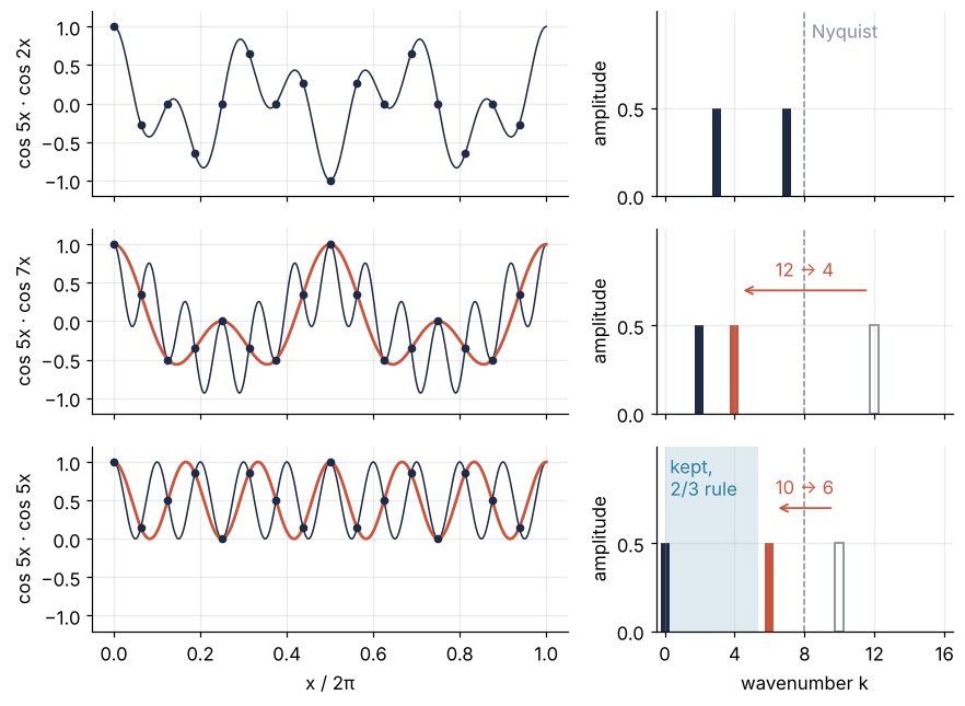
Products of two cosines sampled on 16 points. Left: the product and its samples. Right: its wavenumbers. 5 times 2 gives 3 and 7, below 8; 5 times 7 puts 12 onto 4; 5 times 5 puts 10 onto 6, outside the band up to 5 that the 2/3 rule keeps.

The product \(5 \times 2\) gives 3 and 7, both below 8, and the samples report exactly that. The product \(5 \times 7\) should give 2 and 12; 12 folds to \(16 - 12 = 4\), and the 16 samples are those of \(\tfrac12\cos 2x + \tfrac12 \cos 4x\), the red curve, which is all the FFT can report. The product \(5 \times 5\) should give 0 and 10, and gets 0 and 6. Nothing in the coefficients says which modes are genuine.

Now Burgers. The term \(u\,u_x\) fills wavenumbers up to twice the highest one in \(u\). The sine starts in one mode, and the steepening front pushes energy into ever higher ones:

Show code

top = k >= 17                                           # modes whose products with each other can pass 32
for ti in (0.4, 0.6, 0.8, 1.0):
    e = weight * np.abs(aliased["uh"][round(ti / 0.01)])**2
    print(f"t = {ti}: share of E in modes 17 to 31 = {e[top].sum() / e.sum():.1e}")
i_min = np.argmin(aliased["E"])                         # where the drift turns from loss to gain
for i in (i_min, -1):
    e = weight * np.abs(aliased["uh"][i])**2
    print(f"t = {aliased['t'][i]:.2f}: E/E0 = {aliased['E'][i] / aliased['E0']:6.3f}, "
          f"share of E in modes 17 to 31 = {e[top].sum() / e.sum():.0%}")

t = 0.4: share of E in modes 17 to 31 = 2.8e-13
t = 0.6: share of E in modes 17 to 31 = 3.2e-08
t = 0.8: share of E in modes 17 to 31 = 4.5e-05
t = 1.0: share of E in modes 17 to 31 = 2.7e-03
t = 2.03: E/E0 =  0.675, share of E in modes 17 to 31 = 4%
t = 2.25: E/E0 = 17.472, share of E in modes 17 to 31 = 45%

At t = 0.4 the modes from 17 up, the ones whose products can pass 32, hold \(3 \times 10^{-13}\) of the energy; by t = 1 they hold 3 parts in a thousand. Every product they enter folds partly onto kept modes with the wrong wavenumber. In the exact product, three modes whose wavenumbers add up trade energy among themselves, and the trades cancel; the Formalization shows that they must. A folded contribution belongs to no such trade, so nothing balances the energy it carries, and the 31-mode energy starts to drift.

Nothing fixes the sign of that drift either. On this run the folds take energy out until t = 2.03, when \(E\) is down to 0.675 of its start; then they put it back, and into the top modes, whose share rises from 4 % to 45 % by t = 2.25. The rate at which the folds move energy is cubic in \(u\), where the energy is quadratic, so energy they add speeds up the next addition more than in proportion. That feedback takes \(E\) from 0.675 to 100 times its start in 0.23 time units. The energy of the explosion comes from the same place the loss went: the arithmetic of the grid, not the physics.

The two-thirds rule: leave room for the fold

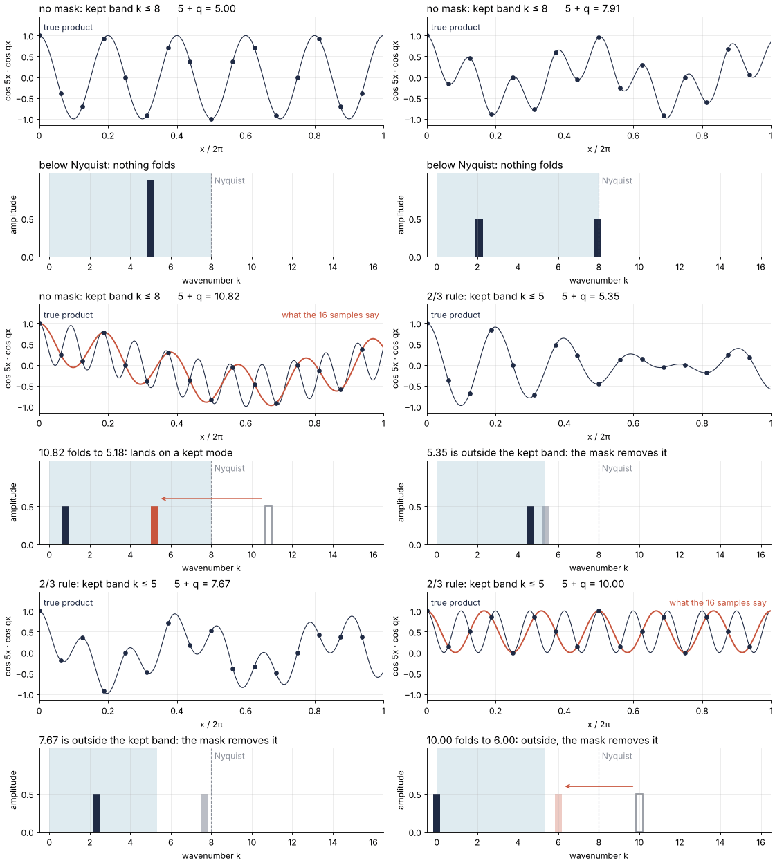
If \(u\) holds only wavenumbers up to \(K\), the product reaches \(2K\), and its fold lands no lower than \(N - 2K\). The fold does no harm if it lands outside the kept band, where it can be thrown away: \(N - 2K > K\), so \(K < N/3\). That is the 2/3 rule (Orszag, 1971): keep the coefficients up to two thirds of the Nyquist wavenumber, set the rest to zero, and zero them again in every product. On 16 points \(K = 5\). The \(5 \times 5\) product of the last figure folds to 6, outside the band, and the mask removes it.

The product cos 5x times cos qx on 16 points as q sweeps up. Top: the true product, its samples, and the slower wave the samples describe once 5 + q passes 8. Bottom: the wavenumber axis; the fold of 5 + q moves left. Without a mask it enters the shaded kept band; under the 2/3 rule it stays outside.

Show code

"""Fold sweep: the product cos(5x) cos(qx) sampled on 16 points, and where its wavenumber 5 + q lands.

First half: no mask, the grid keeps every wavenumber up to the Nyquist value 8, and once 5 + q
passes 8 its fold 16 - (5 + q) lands inside the kept band. Second half: the 2/3 rule keeps k <= 5
only, and the fold stays outside the band, where the mask removes it.
Renders ../../assets/fold-sweep.gif. Run it from any directory:

    python scene.py
"""
from pathlib import Path

import numpy as np
import matplotlib.pyplot as plt
from matplotlib.animation import FuncAnimation, PillowWriter
from PIL import Image

OUT = Path(__file__).resolve().parents[2] / "assets" / "fold-sweep.gif"
INK, ACCENT, SECOND, MUTED = "#1f2a44", "#c8553d", "#2a7f9e", "#8a8f98"
plt.rcParams.update({"axes.spines.top": False, "axes.spines.right": False,
                     "axes.grid": True, "grid.alpha": 0.25, "font.size": 11})

N, P = 16, 5                                       # grid points, the fixed factor's wavenumber
x_fine = np.linspace(0, 2 * np.pi, 600)
x_grid = 2 * np.pi * np.arange(N) / N

# ---- frames: q from 0 to 8 without a mask, then q from 0 to 5 with the 2/3 rule
q_free = np.linspace(0, 8, 56)
q_masked = np.linspace(0, 5, 44)
frames = [(q, 8.0) for q in q_free] + [(q, N / 3) for q in q_masked]

# ---- figure, drawn once
fig, (ax1, ax2) = plt.subplots(2, 1, figsize=(7, 5.2), dpi=80, height_ratios=[1.3, 1],
                               layout="constrained")
(true_line,) = ax1.plot([], [], color=INK, lw=1.0)
(alias_line,) = ax1.plot([], [], color=ACCENT, lw=1.8)
(samples,) = ax1.plot([], [], "o", color=INK, ms=5)
# direct labels in the headroom above y = 1, where both curves start and end
ax1.text(0.08, 1.2, "true product", color=INK, va="center")
alias_label = ax1.text(2 * np.pi - 0.08, 1.2, "what the 16 samples say", color=ACCENT,
                       ha="right", va="center")
ax1.set(xlim=(0, 2 * np.pi), ylim=(-1.15, 1.45), xlabel="x / 2π", ylabel="cos 5x · cos qx",
        xticks=np.linspace(0, 2 * np.pi, 6), xticklabels=["0", "0.2", "0.4", "0.6", "0.8", "1"])
title = ax1.set_title("", loc="left")

band = ax2.axvspan(0, 8, color=SECOND, alpha=0.15, lw=0)
ax2.axvline(N / 2, color=MUTED, ls="--", lw=1)
ax2.text(N / 2 + 0.15, 1.07, "Nyquist", color=MUTED, va="top")
true_bar = ax2.bar([0], [0.5], width=0.35, facecolor="none", edgecolor=MUTED, lw=1.5)[0]
fold_bar = ax2.bar([0], [0.5], width=0.35, lw=0)[0]
low_bar = ax2.bar([0], [0.5], width=0.35, color=INK, lw=0)[0]
arrow = ax2.annotate("", xy=(0, 0.6), xytext=(0, 0.6),
                     arrowprops=dict(arrowstyle="->", color=ACCENT, lw=1.4))
verdict = ax2.set_title("", loc="left")
ax2.set(xlim=(-0.5, 16.5), ylim=(0, 1.1), yticks=[0, 0.5], ylabel="amplitude",
        xticks=range(0, 17, 2), xlabel="wavenumber k")

# ---- one frame: a function of (q, kept band edge) alone
def update(frame):
    q, edge = frame
    s, d = P + q, abs(P - q)
    folds = s > N / 2
    shown = N - s if folds else s                   # where the samples put the sum wavenumber
    true_line.set_data(x_fine, np.cos(P * x_fine) * np.cos(q * x_fine))
    samples.set_data(x_grid, np.cos(P * x_grid) * np.cos(q * x_grid))
    alias = 0.5 * np.cos(d * x_fine) + 0.5 * np.cos(shown * x_fine)
    alias_line.set_data(x_fine, alias)
    alias_line.set_visible(folds)
    alias_label.set_visible(folds)
    band.set_x(0)
    band.set_width(edge)
    true_bar.set_x(s - 0.175)
    true_bar.set_visible(folds)
    low_bar.set_x(d - 0.175)
    fold_bar.set_x(shown - 0.175)
    fold_bar.set_y(0.5 if abs(shown - d) < 0.35 else 0)   # stacked when it lands on the difference
    fold_bar.set_color(ACCENT if folds else INK)            # red only for a wavenumber the grid misplaced
    fold_bar.set_alpha(1.0 if shown <= edge else 0.3)       # faded: outside the kept band
    arrow.xy, arrow.xyann = (shown + 0.25, 0.6), (s - 0.25, 0.6)   # from the true sum to the fold, ends beside the bars
    arrow.set_visible(folds and s - shown > 1.0)
    if edge == 8.0:
        title.set_text(f"no mask: kept band k ≤ 8      5 + q = {s:.2f}")
    else:
        title.set_text(f"2/3 rule: kept band k ≤ 5      5 + q = {s:.2f}")
    if not folds and s <= edge:
        verdict.set_text("below Nyquist: nothing folds")
    elif not folds:
        verdict.set_text(f"{s:.2f} is outside the kept band: the mask removes it")
    elif shown <= edge:
        verdict.set_text(f"{s:.2f} folds to {shown:.2f}: lands on a kept mode")
    else:
        verdict.set_text(f"{s:.2f} folds to {shown:.2f}: outside, the mask removes it")

# ---- render, and read back what was written
OUT.parent.mkdir(exist_ok=True)
FuncAnimation(fig, update, frames=frames).save(OUT, writer=PillowWriter(fps=12))
plt.close(fig)
with Image.open(OUT) as im:
    delay = im.info["duration"]
    print(f"{OUT.name}: {im.width} x {im.height} px, {im.n_frames} frames at {delay} ms, "
          f"{im.n_frames * delay / 1000:.1f} s, {OUT.stat().st_size / 1024:,.0f} kB")

In the first half the grid keeps everything up to 8, and the fold enters the shaded band the moment \(5 + q\) passes 8. In the second half the band ends at \(16/3\), and the fold of the largest product, 10 onto 6, stays outside it. Between the integers the sweep shows values such as \(q = 3.5\), and \(\cos qx\) is then no Fourier mode at all, because it does not repeat after \(2\pi\). The fold still holds at the 16 points, where \(\cos sx\) and \(\cos (16 - s)x\) agree for any \(s = 5 + q\), so those frames are right about the samples and about nothing between them.

On 64 points the rule keeps \(k \le 21\). Here is the Burgers run again, masked:

Show code

masked = run(dealias="2/3")
for name, r in [("no mask ", aliased), ("2/3 rule", masked)]:
    u2 = irfft(r["uh"][i2], N, norm="forward")
    print(f"{name} at t = 2: E/E0 - 1 = {r['E'][i2] / r['E0'] - 1:+.1e}, max |u| = {np.abs(u2).max():.2f}")

no mask  at t = 2: E/E0 - 1 = -3.2e-01, max |u| = 1.10
2/3 rule at t = 2: E/E0 - 1 = -2.2e-15, max |u| = 1.69

At t = 2 the masked run's energy has moved by \(2 \times 10^{-15}\), where the unmasked run has lost 32 %. Its profile overshoots to 1.69, though the true one never leaves \([-1, 1]\); the Formalization comes back to that.

Longer products need more room. With \(m\) factors the product reaches \(mK\), and the same argument gives \(K < N/(m + 1)\). The cubic term of the Cahn-Hilliard tutorial needs \(K < N/4\), which keeps half of the wavenumbers up to Nyquist: the half rule. Either way the rule throws away modes the grid could carry, a third of them for a quadratic term. Padding keeps them.

The question

The idea: a product holds wavenumbers the grid cannot

The two-thirds rule: leave room for the fold

The second half of this tutorial needs a free account