2D turbulence with a pseudo-spectral solver: eddies merge into vortices (Python)

The problem: why do the eddies in a thin layer of fluid merge?

Stir a soap film and the eddies do not break into smaller ones, as they do in a stirred cup of coffee. They merge into fewer, larger vortices. The atmosphere and the ocean do the same at scales of hundreds of kilometers, where the layer is thin compared with its width and the flow nearly two-dimensional; engineers reproduce it in soap-film tunnels and in shallow layers of salt water stirred by magnets. In 1967 Kraichnan predicted that the energy spectrum of such a flow falls as \(E(k) \propto k^{-3}\) in the enstrophy range, the scales between the energy peak and the smallest eddies, through which the squared vorticity flows down to where viscosity removes it.

On a periodic square of side 2π, the vorticity \(\omega = \partial v/\partial x - \partial u/\partial y\) of a velocity field (u, v) obeys

\[\frac{\partial\omega}{\partial t} + u\,\frac{\partial\omega}{\partial x} + v\,\frac{\partial\omega}{\partial y} = \nu\,\nabla^2\omega, \qquad \nabla^2\psi = -\omega, \qquad u = \frac{\partial\psi}{\partial y},\quad v = -\frac{\partial\psi}{\partial x}.\]

Read the first equation as: each fluid parcel carries its vorticity along (left side) while the viscosity ν smooths it out (right side). The streamfunction ψ turns the vorticity back into the velocity that does the carrying.

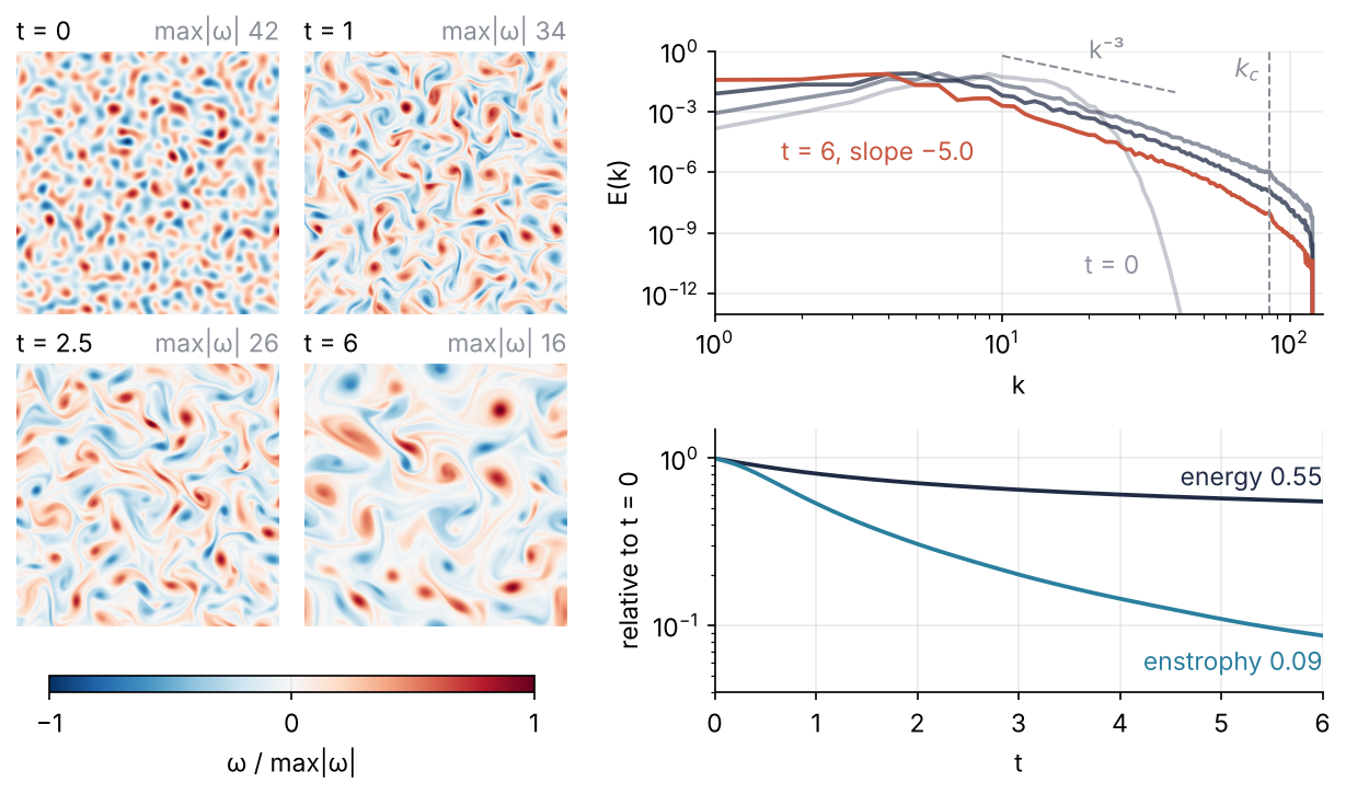
Left: vorticity at t = 0, 1, 2.5, and 6 on the periodic square, red and blue for the two senses of rotation; a fine speckle of eddies becomes fewer, larger vortices. Top right: energy spectra E(k) at those times, the last with slope −5.0 beside a dashed k⁻³ line. Bottom right: energy and enstrophy relative to the start.

This is where we end up. A random field of small eddies on 256 × 256 points organizes within six time units into larger vortices, and the mean wavenumber of the energy falls from 10.5 to 3.7. The final spectrum has a slope of −5.0, steeper than Kraichnan's −3, and the run keeps 55 % of its energy while it loses 91 % of its enstrophy. The main loop takes about 40 s on a laptop. Four pieces make it work: derivatives and the integrating factor from the KdV tutorial, the 2/3 rule now in two dimensions, a Runge-Kutta loop of our own, and a spectrum summed over rings of wavenumber.

Setup

No data to load: Step 4 builds the initial field from random noise with the seed 319. Lengths are in units of the box side over 2π and velocities in units of the initial rms velocity, so the axes carry no units. The grid leaves out x = 2π, which on a periodic domain is x = 0 again. The last number printed says that the initial eddies span 25.6 grid points per wavelength; the eddies the flow makes later are far smaller, which Step 6 checks.

import numpy as np
import matplotlib.pyplot as plt
from functools import cache
from numpy.fft import rfft2, irfft2, fftfreq, rfftfreq

N = 256                  # grid points per side
L = 2 * np.pi            # periodic square [0, 2π)²
NU = 1e-3                # viscosity
K0 = 10                  # peak wavenumber of the initial spectrum
SEED = 319

x = L * np.arange(N) / N
X, Y = np.meshgrid(x, x, indexing="ij")
dx = L / N

plt.rcParams.update({
    "figure.figsize": (7, 3.6), "figure.dpi": 110,
    "axes.spines.top": False, "axes.spines.right": False,
    "axes.grid": True, "grid.alpha": 0.25,
    "font.size": 11, "lines.linewidth": 1.8,
})
INK, ACCENT, SECOND, MUTED = "#1f2a44", "#c8553d", "#2a7f9e", "#8a8f98"
CMAP = "RdBu_r"          # diverging: red and blue for the two senses of rotation

print(f"N = {N}, dx = {dx:.4f}, {2 * np.pi / K0 / dx:.1f} grid points per wavelength at k0 = {K0}")

N = 256, dx = 0.0245, 25.6 grid points per wavelength at k0 = 10

Step 1: Build the wavenumbers and get the velocity from the vorticity

On [0, 2π) the wavenumbers are integers, 2π * fftfreq(N, d=L/N). A real field's coefficient at \(-\mathbf k\) is the complex conjugate of the one at \(\mathbf k\), so rfft2 stores only the half plane \(k_y \ge 0\): axis 0 holds every \(k_x\), both signs, and axis 1 holds \(k_y = 0\) to N/2. norm="forward" works as in KdV. The half plane does not record whether the last axis had an even or an odd length, so irfft2 assumes an even one, 2(m − 1) for m stored columns; s=(n, n) states the length, and without it an odd n comes back one column short. In Fourier space \(\nabla^2\psi = -\omega\) is a division, \(\hat\psi = \hat\omega/k^2\), with the entry at k = 0 set to zero for the reason in the first pitfall. The Taylor-Green vortex \(\omega = 2\kappa\sin\kappa x\sin\kappa y\) has the velocity \(u = \sin\kappa x\cos\kappa y\), \(v = -\cos\kappa x\sin\kappa y\):

@cache                                            # once per grid size; Step 5 uses n = 128
def wavenumbers(n):
    kx = 2 * np.pi * fftfreq(n, d=L / n)          # axis 0: every kx, both signs
    ky = 2 * np.pi * rfftfreq(n, d=L / n)         # axis 1: ky = 0 to n/2 only
    KX, KY = np.meshgrid(kx, ky, indexing="ij")
    K2 = KX**2 + KY**2
    K2inv = np.divide(1, K2, out=np.zeros_like(K2), where=K2 > 0)
    return KX, KY, K2, K2inv

def F(f):
    return rfft2(f, norm="forward")

def Finv(fh):
    n = fh.shape[0]
    return irfft2(fh, s=(n, n), norm="forward")

def velocity(wh):
    KX, KY, _, K2inv = wavenumbers(wh.shape[0])
    psih = wh * K2inv                             # ψ̂ = ω̂/k², zero at k = 0
    return Finv(1j * KY * psih), Finv(-1j * KX * psih)

kappa = 4
w_tg = 2 * kappa * np.sin(kappa * X) * np.sin(kappa * Y)
u, v = velocity(F(w_tg))
err_u = np.abs(u - np.sin(kappa * X) * np.cos(kappa * Y)).max()
err_v = np.abs(v + np.cos(kappa * X) * np.sin(kappa * Y)).max()
print(f"Taylor-Green, κ = {kappa}: max error in u {err_u:.1e}, in v {err_v:.1e}")

Taylor-Green, κ = 4: max error in u 2.1e-15, in v 2.0e-15

Round-off, 2 × 10⁻¹⁵, where a wrong sign in \(\hat\psi\) or in either velocity, or a missing factor of k, would give an error of order one.

Step 2: Compute the advection term on the grid

In Fourier space the product \(u\,\omega_x + v\,\omega_y\) would couple every pair of modes; on the grid it is one multiplication per point, as for KdV's \(u^2\). Four fields go to the grid and one comes back: five FFTs. The mask keep is filled in by Step 5; here it keeps every mode. For Taylor-Green ω is proportional to ψ, and the velocity runs along the contours of ψ, hence along those of ω, so the term vanishes exactly:

def advection(wh, keep):
    KX, KY, _, _ = wavenumbers(wh.shape[0])
    u, v = velocity(wh)
    wx, wy = Finv(1j * KX * wh), Finv(1j * KY * wh)
    return -F(u * wx + v * wy) * keep

keep_all = np.ones(F(w_tg).shape, dtype=bool)
adv = Finv(advection(F(w_tg), keep_all))
print(f"max |u·∇ω| = {np.abs(adv).max():.1e}, against max|u| · max|∇ω| = 2κ² = {2 * kappa**2}")

max |u·∇ω| = 3.5e-13, against max|u| · max|∇ω| = 2κ² = 32

3.5 × 10⁻¹³ against a scale of 32: the two products cancel to round-off, which a sign error between them would spoil.

Step 3: Step in time with RK4 and an integrating factor

KdV's integrating factor works here with a real, negative symbol, \(-\nu k^2\); since \(e^{-\nu k^2 t}\) would underflow over a whole run, each step restarts it at \(t_n\). With \(\mathcal N\) the advection term, \(\hat v = e^{\nu k^2(t - t_n)}\hat\omega\) obeys \(d\hat v/dt = e^{\nu k^2(t - t_n)}\mathcal N(\hat\omega)\). Classical RK4 on \(\hat v\), written back in \(\hat\omega\) with \(E = e^{-\nu k^2\Delta t/2}\), is the integrating-factor RK4 of KdV's Variations:

\[a = \mathcal N(\hat\omega_n),\quad b = \mathcal N\big(E(\hat\omega_n + \tfrac{\Delta t}{2}a)\big),\quad c = \mathcal N\big(E\hat\omega_n + \tfrac{\Delta t}{2}b\big),\quad d = \mathcal N\big(E^2\hat\omega_n + \Delta t\,E c\big),\]

\[\hat\omega_{n+1} = E^2\hat\omega_n + \tfrac{\Delta t}{6}\big(E^2 a + 2E(b + c) + d\big).\]

Each stage evaluates \(\mathcal N\) at \(\hat\omega\), so its slope for \(\hat v\) carries \(1/E\) at mid step and \(1/E^2\) at the end. In b, E turns the mid-step \(\hat v = \hat\omega_n + \tfrac{\Delta t}{2}a\) back into \(\hat\omega\); in c, the \(1/E\) in b's slope cancels that E. The update is \(\hat v_{n+1}\) times \(E^2\).

Advection only turns the phase of a mode \(e^{i\mathbf k\cdot\mathbf x}\), at the rate \(\mathbf u\cdot\mathbf k\). One RK4 step multiplies such a rotation by \(R(z) = 1 + z + z^2/2 + z^3/6 + z^4/24\) with \(z = -i\,\mathbf u\cdot\mathbf k\,\Delta t\), and \(|R| \le 1\) only while \(|\mathbf u\cdot\mathbf k|\,\Delta t \le 2\sqrt2 \approx 2.83\):

def R(z):                                         # one RK4 step on dy/dt = λy, z = λΔt
    return 1 + z + z**2 / 2 + z**3 / 6 + z**4 / 24

for y in [1.5, 2.9]:
    print(f"|R({y}i)| = {abs(R(1j * y)):.2f}, after 1,000 steps {abs(R(1j * y))**1000:.0e}")

|R(1.5i)| = 0.94, after 1,000 steps 6e-27
|R(2.9i)| = 1.19, after 1,000 steps 5e+76

Just below the bound a thousand steps damp the mode to 6 × 10⁻²⁷; just above they amplify it 10⁷⁶-fold. The fastest rotation is the largest speed times the largest kept \(|\mathbf k|\), \(\sqrt2\,k_c \approx 120\) in the corner of Step 5's square mask, so \(\Delta t = C/(\max|\mathbf u|\,\sqrt2\,k_c)\) with the CFL number C = 1.5. The viscous limit is 47 times looser (Step 6), so at ν = 10⁻³ the factor buys exact decay, not a longer step. Taylor-Green has no advection, so at ν = 0.05 the factor alone moves it, as \(e^{-2\nu\kappa^2 t}\):

def time_step(wh, keep, C=1.5):
    u, v = velocity(wh)
    k_max = np.sqrt(wavenumbers(wh.shape[0])[2][keep].max())   # the corner of the mask
    return C / (np.hypot(u, v).max() * k_max)

def rk4_step(wh, dt, nu, keep):
    E = np.exp(-nu * wavenumbers(wh.shape[0])[2] * dt / 2)       # the factor over half a step
    a = advection(wh, keep)
    b = advection(E * (wh + dt / 2 * a), keep)
    c = advection(E * wh + dt / 2 * b, keep)
    d = advection(E**2 * wh + dt * E * c, keep)
    return E**2 * wh + dt / 6 * (E**2 * a + 2 * E * (b + c) + d)

wh = F(w_tg)
for _ in range(100):
    wh = rk4_step(wh, 0.01, 0.05, keep_all)
amp, exact = Finv(wh).max() / (2 * kappa), np.exp(-2 * 0.05 * kappa**2 * 1.0)
print(f"amplitude at t = 1: {amp:.12f}, exp(-2νκ²t) = {exact:.12f}, relative error {abs(amp / exact - 1):.0e}")

amplitude at t = 1: 0.201896517995, exp(-2νκ²t) = 0.201896517995, relative error 2e-15

Round-off again, 2 × 10⁻¹⁵ relative: the exponent is right, and one step advances the factor by Δt, not Δt/2.

Step 4: Start from a random field and measure its spectrum by shells

The energy spectrum E(k) sums ½|û|² = ½|ω̂|²/k² over the modes of a ring, round(\(|\mathbf k|\)) = k, with np.bincount. Each stored column with \(k_y > 0\) also stands for its conjugate partner at \(-\mathbf k\), which has the same energy, so it counts twice. The columns \(k_y = 0\) and \(k_y = N/2\) hold their own partners, whose mirror images lie in the same column, so they count once. The energy is the sum of the spectrum, the enstrophy \(Z = \tfrac12\langle\omega^2\rangle = \sum k^2 E(k)\) the same sum with \(k^2\), and \(\bar k = \sum k\,E(k)/\sum E(k)\) the size of the eddies as one number.

def weights(n):
    W = np.full(n // 2 + 1, 2.0)                  # column ky > 0 also stands for its partner at -k
    W[[0, -1]] = 1                                # ky = 0 and ky = n/2 hold their own partners
    return W

def spectrum(wh):
    n = wh.shape[0]
    _, _, K2, K2inv = wavenumbers(n)
    e = 0.5 * weights(n) * np.abs(wh)**2 * K2inv  # ½|û|², since |û| = |ω̂|/k
    shell = np.rint(np.sqrt(K2)).astype(int)
    return np.bincount(shell.ravel(), e.ravel())  # E(k) for k = 0, 1, 2, ...

def energy(wh):
    return spectrum(wh).sum()

def enstrophy(wh):                                # Σ k² E(k), mode by mode
    return (0.5 * weights(wh.shape[0]) * np.abs(wh)**2).sum()

def mean_k(E_k):
    return (np.arange(E_k.size) * E_k).sum() / E_k.sum()

To build a field with a given spectrum, turn the sum around. A ring of radius k holds about 2πk modes, so with the same |û| in each, \(E(k) \approx 2\pi k\cdot\tfrac12|\hat u|^2\), and each mode needs \(|\hat\omega| = k|\hat u| = \sqrt{k E(k)/\pi}\). The target is \(E(k) \propto (k/k_0)^4 e^{-2(k/k_0)^2}\) with \(k_0 = 10\). The transform of real white noise times that amplitude has the conjugate symmetry for free; the mean is removed and E set to 0.5:

def initial_field(n, seed=SEED):
    k = np.sqrt(wavenumbers(n)[2])
    E_target = (k / K0)**4 * np.exp(-2 * (k / K0)**2)
    noise = F(np.random.default_rng(seed).standard_normal((n, n)))
    wh = noise * np.sqrt(k * E_target / np.pi)    # |ω̂| = sqrt(k E(k)/π)
    wh[0, 0] = 0
    return wh * np.sqrt(0.5 / energy(wh))         # E = 0.5, rms velocity 1

wh0 = initial_field(N)
u0, v0 = velocity(wh0)
E_spec, E_grid = energy(wh0), 0.5 * np.mean(u0**2 + v0**2)
print(f"E from the shells {E_spec:.6f}, from the grid {E_grid:.6f}, difference {abs(E_spec - E_grid):.0e}")
print(f"Z = {enstrophy(wh0):.1f} (smooth spectrum: 5/4 k0² E = {5 / 4 * K0**2 * 0.5:.1f}), "
      f"peak shell k = {spectrum(wh0).argmax()}, k̄ = {mean_k(spectrum(wh0)):.2f}, max|u| = {np.hypot(u0, v0).max():.2f}")

E from the shells 0.500000, from the grid 0.500000, difference 0e+00
Z = 61.8 (smooth spectrum: 5/4 k0² E = 62.5), peak shell k = 9, k̄ = 10.49, max|u| = 3.02

The two energies agree to every printed digit, which checks the weights. Z = 61.8 against 62.5 for the smooth spectrum, and the noise moves the peak to k = 9.

Step 5: Dealias with the 2/3 rule, and see what aliasing does without it

Without viscosity, advection carries each parcel's vorticity around without changing it, so neither the enstrophy Z nor, as in any frictionless flow, the energy E can change. In three dimensions vortex stretching breaks the first; in two there is nothing to stretch. With \(Z = \sum k^2 E(k)\), a nonlinear term that spreads the spectrum cannot move energy to large k without raising Z. So on balance energy moves to small k, into larger eddies, and enstrophy to large k, where viscosity removes it. That is Fjørtoft's argument: the bookkeeping, not a force, makes the eddies merge.

The discrete equations keep both invariants only when dealiased. In two dimensions each axis folds on its own, so KdV's 2/3 rule applies per axis, and the mask is a square:

def dealias_mask(n):
    KX, KY, _, _ = wavenumbers(n)
    k_c = 2 / 3 * (n // 2)
    return (np.abs(KX) < k_c) & (np.abs(KY) < k_c)

KEEP = dealias_mask(N)
print(f"{KEEP[0, 1:].sum()} of {N // 2} positive wavenumbers per axis kept, {KEEP.mean():.1%} of the stored modes")

85 of 128 positive wavenumbers per axis kept, 44.5% of the stored modes

With the mask, what the product puts beyond the cut is discarded, and the kept modes obey the true equations. Without it, that part lands on kept modes with the wrong wavenumber. The test runs ν = 0 at N = 128 to t = 5, with the mask at two time steps and without it. run records the spectrum and Z every ten steps.

def run(wh0, T, dt, nu, keep, every=10, snapshots=()):
    wh = keep * wh0
    t, spec, Z, snaps = [0.0], [spectrum(wh)], [enstrophy(wh)], {}
    at_step = {round(ts / dt): ts for ts in snapshots}
    if 0 in at_step:
        snaps[0] = wh
    steps = round(T / dt)
    for n in range(1, steps + 1):
        wh = rk4_step(wh, dt, nu, keep)
        if n in at_step:
            snaps[at_step[n]] = wh
        if n % every == 0 or n == steps:
            t.append(n * dt)
            spec.append(spectrum(wh))
            Z.append(enstrophy(wh))
            if Z[-1] > 10 * Z[0]:                 # enstrophy cannot grow: the run has blown up
                break
    return np.array(t), np.array(spec), np.array(Z), snaps

n = 128
wh_small = initial_field(n)
keep_small = dealias_mask(n)
dt_small = time_step(keep_small * wh_small, keep_small)
tests = {}
for label, keep, dt in [("2/3 rule", keep_small, dt_small),
                        ("2/3 rule, Δt/2", keep_small, dt_small / 2),
                        ("no mask", np.ones_like(keep_small), dt_small)]:
    t, spec, Z, _ = run(wh_small, 5, dt, 0.0, keep)
    E = spec.sum(axis=1)
    tests[label] = t, np.abs(E / E[0] - 1), np.abs(Z / Z[0] - 1)
    print(f"{label:15s} max |ΔE|/E₀ = {tests[label][1].max():.1e}, "
          f"max |ΔZ|/Z₀ = {tests[label][2].max():.1e}, until t = {t[-1]:.2f}")

2/3 rule        max |ΔE|/E₀ = 3.8e-04, max |ΔZ|/Z₀ = 4.9e-03, until t = 5.00
2/3 rule, Δt/2  max |ΔE|/E₀ = 1.2e-05, max |ΔZ|/Z₀ = 1.6e-04, until t = 5.00
no mask         max |ΔE|/E₀ = 4.4e-01, max |ΔZ|/Z₀ = 1.0e+01, until t = 0.28

Show code

fig, axes = plt.subplots(2, 1, sharex=True, figsize=(7, 4.2))
alpha = {"2/3 rule": 1, "2/3 rule, Δt/2": 0.45, "no mask": 1}
for ax, quantity, color in zip(axes, (1, 2), (INK, SECOND)):   # energy in INK, enstrophy in SECOND, as in Step 6
    for label, run_data in tests.items():
        t, d = run_data[0], run_data[quantity]
        ax.semilogy(t[1:], d[1:], color=color, alpha=alpha[label])
        if label != "no mask":                    # name the masked runs at their right end
            ax.text(5.08, d[-1], label, color=color, alpha=alpha[label], va="center")
t_blow = tests["no mask"][0][-1]
axes[0].text(t_blow + 0.1, 0.3, "no mask", color=INK, va="center")
axes[1].text(t_blow + 0.1, 3, f"no mask: Z > 10 Z₀ at t = {t_blow:.2f}", color=SECOND, va="center")
axes[0].set(ylabel="|ΔE| / E₀", ylim=(1e-11, 10))
axes[1].set(ylabel="|ΔZ| / Z₀", xlabel="t", xlim=(0, 5), ylim=(1e-9, 1e2))
plt.show()

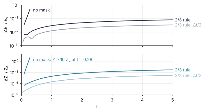
Relative change of energy (top) and enstrophy (bottom) against t in inviscid runs, log scale. Without the mask both reach order one by t = 0.28; with the 2/3 rule they stay below 10⁻³ and 10⁻², and halving the time step lowers them about thirtyfold.

Without the mask Z grows more than tenfold by t = 0.28, which the true equations forbid. With it E drifts by 4 × 10⁻⁴ and Z by 5 × 10⁻³, and halving Δt cuts both about 31-fold, not the 16 of a fourth-order method. RK4 errs in the phase of a rotating mode at fourth order but in its amplitude, which E and Z measure, at fifth: \(|R(iy)|^2 = 1 - y^6/72 + y^8/576\), a loss of \(y^6/72\) per step and of order \(\Delta t^5\) over the \(1/\Delta t\) steps of one time unit. So the drift is the time stepping's.

Step 6: Run the decay, fit the slope, and draw the result

The main run steps the 256² field at ν = 10⁻³ to t = 6 with Step 3's Δt and keeps four snapshots. It prints the CFL number at both ends, since the step was fixed at the start, and the resolution check, the energy at the cutoff relative to the peak at the worst output:

T = 6
dt = time_step(KEEP * wh0, KEEP)
t, spec, Z, snaps = run(wh0, T, dt, NU, KEEP, snapshots=(0, 1, 2.5, T))
E = spec.sum(axis=1)
k_c = KEEP[0, 1:].sum()
k_max = np.sqrt(2) * k_c                          # the corner of the square mask
tail = spec[:, k_c] / spec.max(axis=1)
C0, CT = [np.hypot(*velocity(snaps[ts])).max() * k_max * dt for ts in (0, T)]
print(f"{round(T / dt)} steps of Δt = {dt:.5f}, CFL number {C0:.2f} at t = 0 and {CT:.2f} at t = {T}")
print(f"explicit RK4 on the viscous term alone would allow Δt = {2.785 / (NU * k_max**2):.3f}")   # stable down to -2.785
print(f"E(T)/E(0) = {E[-1] / E[0]:.3f}, Z(T)/Z(0) = {Z[-1] / Z[0]:.3f}")
print(f"k̄ from {mean_k(spec[0]):.2f} to {mean_k(spec[-1]):.2f}, peak shell at t = {T}: k = {spec[-1].argmax()}")
print(f"E(k_c)/E(peak), worst over {len(t)} outputs: {tail.max():.1e} at t = {t[tail.argmax()]:.2f}")

1454 steps of Δt = 0.00413, CFL number 1.50 at t = 0 and 0.89 at t = 6
explicit RK4 on the viscous term alone would allow Δt = 0.193
E(T)/E(0) = 0.551, Z(T)/Z(0) = 0.087
k̄ from 10.49 to 3.69, peak shell at t = 6: k = 4
E(k_c)/E(peak), worst over 147 outputs: 3.3e-05 at t = 0.58

Energy keeps 55 %, enstrophy 9 %, and \(\bar k\) falls from 10.5 to 3.7: Step 5's bookkeeping, with viscosity taking the enstrophy that reached small scales. The CFL number falls to 0.89 as the flow slows. The worst moment for resolution is t = 0.58, the first burst of enstrophy toward small scales, and even then the cutoff sits 4.5 decades below the peak. The slope fit runs over 10 ≤ k ≤ 40, above the final peak at k = 4 and below the viscous bend:

k = np.arange(spec.shape[1])

def slope(E_k, lo, hi):
    s = slice(lo, hi + 1)
    return np.polyfit(np.log(k[s]), np.log(E_k[s]), 1)[0]

for lo, hi in [(10, 40), (10, 20), (20, 40)]:
    print(f"slope of E(k) at t = {T}, {lo} ≤ k ≤ {hi}: {slope(spec[-1], lo, hi):.2f}")

slope of E(k) at t = 6, 10 ≤ k ≤ 40: -5.05
slope of E(k) at t = 6, 10 ≤ k ≤ 20: -4.97
slope of E(k) at t = 6, 20 ≤ k ≤ 40: -5.36

−5.05, steeper than Kraichnan's −3. That is the documented outcome of decaying runs, not a solver error: coherent vortices form, and McWilliams (1984) found spectra this steep in such simulations.

Show code

fig = plt.figure(figsize=(8, 4.6))
W, H = 8, 4.6
def place(x, y, w, h):                            # an axes at a position given in inches
    return fig.add_axes([x / W, y / H, w / W, h / H])

times = sorted(snaps)
for j, ts in enumerate(times):                    # a 2 × 2 block of snapshots, each scaled by its own max|ω|
    ax = place(1.75 * (j % 2), 2.85 - 1.9 * (j // 2), 1.6, 1.6)
    w = Finv(snaps[ts])
    im = ax.imshow(w.T / np.abs(w).max(), origin="lower", cmap=CMAP, vmin=-1, vmax=1)
    ax.set_axis_off()
    ax.text(0, 1.02, f"t = {ts:g}", transform=ax.transAxes, va="bottom")
    ax.text(1, 1.02, f"max|ω| {np.abs(w).max():.0f}", transform=ax.transAxes, va="bottom", ha="right", color=MUTED)
fig.colorbar(im, cax=place(0.2, 0.55, 2.95, 0.1), orientation="horizontal", label="ω / max|ω|", ticks=[-1, 0, 1])

ax_s, ax_t = place(4.25, 2.85, 3.7, 1.6), place(4.25, 0.55, 3.7, 1.6)
for j, ts in enumerate(times):
    i = np.argmin(np.abs(t - ts))
    last = j == len(times) - 1
    ax_s.loglog(k[1:], spec[i, 1:], color=ACCENT if last else INK, alpha=1 if last else 0.25 + 0.25 * j)
fit = slope(spec[-1], 10, 40)
kk = np.array([10, 40])
ref = 300 * spec[-1, 10] * (kk / 10)**-3.0        # a k⁻³ guide over the fit range, above the curves
ax_s.loglog(kk, ref, color=MUTED, ls="--", lw=1)
ax_s.text(np.sqrt(kk.prod()), 3 * np.sqrt(ref.prod()), "k⁻³", color=MUTED, va="bottom")
ax_s.axvline(k_c, color=MUTED, ls="--", lw=1)
ax_s.text(k_c / 1.08, 0.05, "$k_c$", color=MUTED, ha="right")
ax_s.text(8, spec[-1, 10] / 30, f"t = {T:g}, slope {fit:.1f}".replace("-", "−"), color=ACCENT, ha="right", va="top")
ax_s.text(30, 1e-11, "t = 0", color=INK, alpha=0.5, ha="right")
ax_s.set(xlabel="k", ylabel="E(k)", xlim=(1, 130), ylim=(1e-13, 1))

ax_t.semilogy(t, E / E[0], color=INK)
ax_t.semilogy(t, Z / Z[0], color=SECOND)
ax_t.text(T, E[-1] / E[0] * 1.15, f"energy {E[-1] / E[0]:.2f}", color=INK, ha="right", va="bottom")
ax_t.text(T, Z[-1] / Z[0] / 1.15, f"enstrophy {Z[-1] / Z[0]:.2f}", color=SECOND, ha="right", va="top")
ax_t.set(xlabel="t", ylabel="relative to t = 0", xlim=(0, T), ylim=(0.04, 1.5))
plt.show()

Left: vorticity at t = 0, 1, 2.5, and 6 on the periodic square, red and blue for the two senses of rotation; a fine speckle of eddies becomes fewer, larger vortices. Top right: energy spectra E(k) at those times, the last with slope −5.0 beside a dashed k⁻³ line. Bottom right: energy and enstrophy relative to the start.

Each snapshot is scaled by its own max|ω|, which falls from 42 to 16, so the colors compare shapes. RdBu_r is diverging, white for no rotation; the colormaps tutorial says why a signed field needs one. The speckle at t = 0 has become fewer, rounder vortices by t = 6, joined by thin filaments where the enstrophy goes to be dissipated.

Pitfalls

Dividing by k² at k = 0. Write psih = wh / K2 and the first call prints a RuntimeWarning, and u and v come back as NaN at every point: the entry at k = 0 is 0/0, and the inverse transform spreads the NaN everywhere. That entry is the mean of ψ, which the velocity never sees, since it only takes derivatives of ψ. Set it to zero, as K2inv does once. The mean vorticity on a periodic domain is zero anyway, because it is the integral of a derivative over a period.

A viscosity too small for the grid. The enstrophy cascade reaches the cutoff before viscosity removes it, and the mask keeps the run stable, so nothing blows up to warn you. The symptom is in the spectrum, which flattens or turns up just below \(k_c\), and in the vorticity, as ripples at the grid scale around the edges of the vortices. A short run at ν/10 through the worst moment shows the first, measured at the output where the tail is highest:

def tail_check(spec):                             # at the output where the tail is highest
    i = (spec[:, k_c] / spec.max(axis=1)).argmax()
    return spec[i, k_c] / spec[i].max(), slope(spec[i], 70, k_c)

_, spec_low, _, _ = run(wh0, 0.8, dt, NU / 10, KEEP)
for nu, sp in [(NU, spec), (NU / 10, spec_low)]:
    ratio, steep = tail_check(sp)
    print(f"ν = {nu:g}: E(k_c)/E(peak) up to {ratio:.1e}, slope over 70 ≤ k ≤ {k_c}: {steep:.1f}")

ν = 0.001: E(k_c)/E(peak) up to 3.3e-05, slope over 70 ≤ k ≤ 85: -4.1
ν = 0.0001: E(k_c)/E(peak) up to 3.0e-04, slope over 70 ≤ k ≤ 85: -1.0

At ν = 10⁻³ the spectrum still falls as \(k^{-4.1}\) into the cutoff; at a tenth of that it flattens to \(k^{-1.0}\), and the energy at the cutoff rises ninefold, to 3.0 × 10⁻⁴ of the peak against 3.3 × 10⁻⁵. Raise ν or N until Step 6's printed ratio and this slope come back.

Fitting the slope where there is no range. The symptom is a slope that moves by more than 0.5 when you move the fit range. At small k a ring holds only 2πk modes, a handful, so E(k) is noisy there; at large k viscosity bends it down. Fit between the peak and the roll-off and report the two half ranges. Here they give −4.97 for 10 ≤ k ≤ 20 and −5.36 for 20 ≤ k ≤ 40, 0.4 apart, so the range is real and steepens slightly with k. For a smoother spectrum, average it over the last few outputs before fitting.

Variations

Forced turbulence and the dual cascade. Add a forcing confined to a band of wavenumbers around \(k_f\) and a linear drag \(-\mu\omega\) to the right-hand side. In the steady state energy runs to large scales with \(E \propto k^{-5/3}\) below \(k_f\) and enstrophy to small scales with \(k^{-3}\) above it, which is Kraichnan's prediction proper.
The beta plane. Add \(\beta v\) to the left-hand side, the change of the Coriolis parameter with latitude. In Fourier space it becomes \(+i\beta k_x\hat\omega/k^2\) on the right, linear and imaginary, so it joins the integrating factor. The vortices give way to Rossby waves and zonal jets.
Hyperviscosity. Replace \(\nu\nabla^2\omega\) by \(-\nu_4\nabla^4\omega\), with the factor \(e^{-\nu_4 k^4 t}\). It removes enstrophy only near the cutoff, so the enstrophy range grows longer at the same N, and an explicit step limit would now shrink like \(k_{\max}^{-4}\). Here the integrating factor buys the step, for the reason the stiffness tutorial gives.
Faster transforms. scipy.fft.rfft2 and irfft2 take the same arguments plus workers=-1, which spreads one transform over every core. Switch before raising N: on a four-core machine they ran two to three times faster than numpy.fft on one core, and workers=-1 about doubled that from N = 512 on.

Cheat sheet

KX, KY = np.meshgrid(2*np.pi*fftfreq(N, d=L/N), 2*np.pi*rfftfreq(N, d=L/N), indexing="ij")
K2 = KX**2 + KY**2
K2inv = np.divide(1, K2, out=np.zeros_like(K2), where=K2 > 0)   # zero at k = 0, not NaN
keep = (abs(KX) < 2/3*(N//2)) & (abs(KY) < 2/3*(N//2))          # 2/3 rule per axis: a square
F = lambda f: rfft2(f, norm="forward"); Finv = lambda fh: irfft2(fh, s=(N, N), norm="forward")
psih = wh*K2inv; u, v = Finv(1j*KY*psih), Finv(-1j*KX*psih)    # streamfunction, then velocity
Nh = -F(u*Finv(1j*KX*wh) + v*Finv(1j*KY*wh))*keep               # advection: five FFTs
E = np.exp(-nu*K2*dt/2)                                         # factor over half a step, restarted each step
wh = E**2*wh + dt/6*(E**2*a + 2*E*(b + c) + d)                  # IF-RK4 from the stages a, b, c, d
dt = 1.5/(max_speed*np.sqrt(2)*k_c)                             # |u·k| dt < 2√2, corner of the mask