Cahn-Hilliard with a semi-implicit spectral step: how fast domains grow (Python)

The problem: how fast do the domains of a quenched blend grow?

Quench a 50:50 polymer blend from above its mixing temperature to below it, and it separates. A fine labyrinth of A-rich and B-rich domains appears, then coarsens: small domains dissolve, and their material diffuses to the larger ones. A binary alloy does the same, and in scaled units the Cahn-Hilliard equation describes both,

\[\frac{\partial c}{\partial t} = \nabla^2\mu, \qquad \mu = c^3 - c - \kappa\nabla^2 c ,\]

with c the composition, −1 for pure A and +1 for pure B. The chemical potential μ is the derivative of the mixing free energy with respect to c, and the first equation is Fick's law with μ in place of the concentration: material flows down the gradient of μ, which inside the unstable mixture means uphill in c. The term c³ − c comes from a double-well free energy with minima at the phases c = ±1, and −κ∇²c charges for interfaces.

Why should the domains grow as t^⅓? The curved interface of a domain of size R raises its chemical potential by an amount ∝ 1/R, the Gibbs-Thomson effect that makes small droplets evaporate first. That difference drives diffusion over a distance ∝ R, so dR/dt ∝ 1/R², and R³ ∝ t.

The fourth derivative hidden in ∇²μ makes the equation stiff. On a 256 by 256 grid an explicit step must stay below 0.0024 time units, about two million steps to t = 5,000. In Fourier space the stiff part becomes a division per mode, which buys a step 800 times larger for one rfft2 and one irfft2 per step.

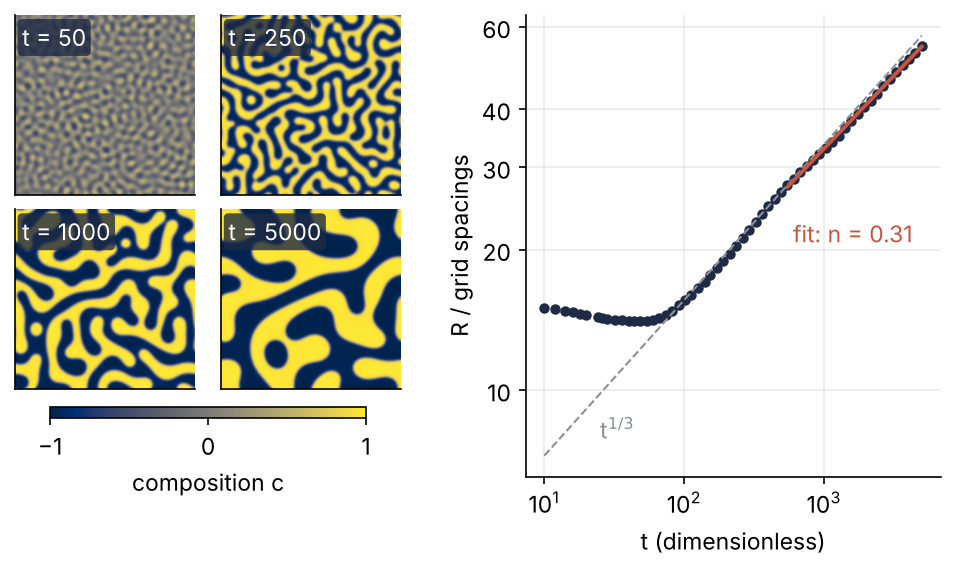
Left: the blend at t = 50, 250, 1000 and 5000, a fine labyrinth coarsening into wide domains. Right: domain size R against time on log axes; the fitted slope n = 0.31 runs just below the dashed t^1/3 line.

The domains end four times wider than at t = 50, and the fitted exponent is 0.31 against the expected 1/3. Step 6 draws it.

Setup

Everything is in scaled units: lengths are counted in grid spacings, and time and c are dimensionless. The initial state is the mixture just after the quench, c = 0 with noise of standard deviation 0.02. A flat interface between the phases has the profile c = tanh(x/√(2κ)), and its core, from c = −0.76 to +0.76, is 2√(2κ) wide. The last number printed is that width in grid points; Step 4 shows why it must be at least four.

import numpy as np
import matplotlib.pyplot as plt
from numpy.fft import rfft2, irfft2, rfftfreq, fftfreq

N = 256                  # grid points per side
L = 256.0                # side of the periodic square, so dx = 1
dx = L / N
KAPPA = 2.0              # interface energy coefficient
DT = 2.0                 # time step
T = 5000.0               # end of the run

rng = np.random.default_rng(112)
c0 = 0.02 * rng.standard_normal((N, N))      # the mixture just after the quench

plt.rcParams.update({
    "figure.figsize": (7, 3.6), "figure.dpi": 110,
    "axes.spines.top": False, "axes.spines.right": False,
    "axes.grid": True, "grid.alpha": 0.25,
    "font.size": 11, "lines.linewidth": 1.8,
})
INK, ACCENT, SECOND, MUTED = "#1f2a44", "#c8553d", "#2a7f9e", "#8a8f98"

print(f"c0: mean {c0.mean():+.1e}, std {c0.std():.4f}")
print(f"grid points across the interface core: {2 * np.sqrt(2 * KAPPA) / dx:.1f}")

c0: mean -8.7e-05, std 0.0201
grid points across the interface core: 4.0

Step 1: Build the wavenumbers and measure a pattern's length

A periodic field on the grid is a sum of Fourier modes \(e^{i(k_x x + k_y y)}\). Differentiating a mode once in x multiplies it by \(ik_x\), so the Laplacian, twice in x plus twice in y, multiplies it by \(-(k_x^2 + k_y^2) = -k^2\). The k here are in radians per length, 2π times the cycles per length that fftfreq and rfftfreq return.

rfft2 of a real N × N field keeps N × (N/2 + 1) coefficients. Axis 0 holds every wavenumber in fftfreq order, axis 1 only the nonnegative ones from rfftfreq: for a real field the negative half mirrors the positive half.

The same coefficients measure the pattern. The structure factor \(S(\mathbf k) = |\hat c(\mathbf k)|^2\) says how much of the field repeats with wavelength \(2\pi/|\mathbf k|\), so its weighted mean wavelength

\[R = 2\pi\,\frac{\sum_{\mathbf k} S(\mathbf k)/|\mathbf k|}{\sum_{\mathbf k} S(\mathbf k)}\]

is the typical spacing of the domains, the domain size of this tutorial. Columns 1 to N/2 − 1 of the half plane stand for themselves and their mirrors, so they count twice, and k = 0, the mean of c, is left out. A test field checks both pieces: \(\cos(2\pi\cdot 3x/L)\sin(2\pi\cdot 5y/L)\) has the Laplacian \(-34\,(2\pi/L)^2\) times itself and the single wavelength \(L/\sqrt{34}\).

kx = 2 * np.pi * fftfreq(N, d=dx)             # radians per length, all signs
ky = 2 * np.pi * rfftfreq(N, d=dx)            # nonnegative half only
KX, KY = np.meshgrid(kx, ky, indexing="ij")
k2 = KX**2 + KY**2
kabs = np.sqrt(k2)

w = np.full(k2.shape, 2.0)                    # columns that stand for their mirror image too
w[:, 0] = w[:, -1] = 1.0
w[0, 0] = 0.0                                 # the mean of c is not part of the pattern
kinv = np.divide(1.0, kabs, out=np.zeros_like(kabs), where=kabs > 0)

def domain_size(ch):
    S = w * np.abs(ch)**2
    return 2 * np.pi * (S * kinv).sum() / S.sum()

x = np.arange(N) * dx
X, Y = np.meshgrid(x, x, indexing="ij")
f = np.cos(2 * np.pi * 3 * X / L) * np.sin(2 * np.pi * 5 * Y / L)
lap_exact = -34 * (2 * np.pi / L)**2 * f
lap = irfft2(-k2 * rfft2(f), s=f.shape)
print(f"coefficients: {k2.shape}")
print(f"Laplacian error relative to its amplitude: {np.abs(lap - lap_exact).max() / np.abs(lap_exact).max():.1e}")
print(f"R = {domain_size(rfft2(f)):.2f}, L/sqrt(34) = {L / np.sqrt(34):.2f}")

coefficients: (256, 129)
Laplacian error relative to its amplitude: 4.4e-13
R = 43.90, L/sqrt(34) = 43.90

The Laplacian is right to 4 × 10⁻¹³, which is rounding, and R returns the wavelength of the test field to every digit shown. irfft2 needs s=f.shape: from 129 columns alone it cannot know whether the field had 256 or 257.

Step 2: Measure why an explicit step fails

Transform the equation, and every mode obeys

\[\frac{d\hat c}{dt} = -k^2\,\mathcal F[c^3 - c] - \kappa k^4\,\hat c .\]

The cube stays in real space, where it is one pointwise power; in Fourier space it would couple every mode with every pair of others.

Just after the quench c is near 0, where the slope of c³ − c, 3c² − 1, is −1, so each mode obeys dĉ/dt = (k² − κk⁴)ĉ. Every mode with k² < 1/κ grows, fastest at k² = 1/(2κ), a wavelength of 2π√(2κ) ≈ 13 grid spacings. That growth is the phase separation itself.

Near a bulk phase, c = ±1, the slope is 2, and every mode decays as dĉ/dt = −(2k² + κk⁴)ĉ. This case sets the step: within a few hundred time units the field is ±1 except on the interfaces, and at the large k that set the limit, κk⁴ dominates anyway. One forward Euler step multiplies a mode by g = 1 − Δt(2k² + κk⁴), and |g| exceeds 1, a growth the equation does not have, once Δt(2k² + κk⁴) > 2. This is the per-mode version of the limit in the heat equation tutorial, but it falls like Δx⁴ instead of Δx². The equation is stiff: the fastest modes set the step, although they decay away at once.

dt_max = 2 / (2 * k2 + KAPPA * k2**2).max()
print(f"explicit bound {dt_max:.5f}, steps to t = {T:.0f}: {T / dt_max:,.0f}")

c, dt, history = c0.copy(), 2 * dt_max, []
while not history or history[-1] < 1e6:       # stop before the numbers overflow
    ch = rfft2(c)
    c = irfft2(ch - dt * (k2 * rfft2(c**3 - c) + KAPPA * k2**2 * ch), s=c.shape)
    history.append(np.abs(c).max())
print("at twice the bound, max |c| per step:", " ".join(f"{m:.2g}" for m in history))

explicit bound 0.00244, steps to t = 5000: 2,046,878
at twice the bound, max |c| per step: 0.065 0.073 0.11 0.2 0.4 0.87 2 5.2 23 1.1e+03 9.4e+07

At twice the bound of 0.0024 the field more than doubles at every step after the first few and passes 10⁶ at step 11.

Step 3: Take the stiff term implicitly

Put the stiff term at the new time and leave the cube at the old one:

\[\frac{\hat c^{\,n+1} - \hat c^{\,n}}{\Delta t} = -k^2\,\mathcal F[(c^n)^3 - c^n] - \kappa k^4\,\hat c^{\,n+1} .\]

Collected, the unknown is

\[\hat c^{\,n+1} = \frac{\hat c^{\,n} - \Delta t\,k^2\,\mathcal F[(c^n)^3 - c^n]}{1 + \Delta t\,\kappa k^4} .\]

An implicit step usually means a matrix solve. Here the operator is diagonal in Fourier space, so the solve is a division per mode. That is the rule to carry to your own PDE: the stiff linear part implicit, the nonlinear part explicit, and the division works only when the linear part has constant coefficients.

For a bulk mode the factor per step is \(g = (1 - 2\Delta t\,k^2)/(1 + \Delta t\,\kappa k^4)\). It never exceeds 1, and it stays above −1 as long as Δt(2k² − κk⁴) ≤ 2. The left side is largest at k² = 1/κ, where it equals Δt/κ, so the linearized step is stable for Δt ≤ 2κ = 4, on any grid. Δt = 2 is half that. Near c = 0, g exceeds 1 for k² < 1/κ, as it should: those modes separate the blend. At k = 0 the factor k² removes the update, so the mean of c, the total amount of B, never changes.

Stable is not accurate. Run to t = 1,000 at Δt = 2 and at Δt = 0.5, without dealiasing for now, and compare:

def step(ch, dt=DT, kappa=KAPPA, keep=None):
    c = irfft2(ch, s=(N, N))
    nonlinear = rfft2(c**3 - c)
    if keep is not None:
        nonlinear *= keep
    return (ch - dt * k2 * nonlinear) / (1 + dt * kappa * k2**2)

def run(nsteps, dt=DT, kappa=KAPPA, keep=None):
    ch = rfft2(c0) if keep is None else keep * rfft2(c0)
    for _ in range(nsteps):
        ch = step(ch, dt, kappa, keep)
    return ch

ch_2 = run(500, dt=2.0)
ch_05 = run(2000, dt=0.5)
c_2, c_05 = irfft2(ch_2, s=(N, N)), irfft2(ch_05, s=(N, N))
R_2, R_05 = domain_size(ch_2), domain_size(ch_05)
print(f"R at t = 1000: dt = 2 gives {R_2:.2f}, dt = 0.5 gives {R_05:.2f}, difference {abs(R_2 / R_05 - 1):.2%}")
print(f"change of the mean of c: {c_2.mean() - c0.mean():+.1e}")
print(f"c between {c_2.min():.3f} and {c_2.max():.3f}; largest pointwise difference of the two runs {np.abs(c_2 - c_05).max():.2f}")

R at t = 1000: dt = 2 gives 32.67, dt = 0.5 gives 32.61, difference 0.19%
change of the mean of c: +1.0e-18
c between -1.025 and 1.038; largest pointwise difference of the two runs 2.02

The domain sizes agree to 0.2 %, the mean has moved only by rounding, and c has saturated within 4 % of ±1. The two fields are nonetheless different labyrinths: small differences in the early instability pick different domains to survive. Only the statistics converge, so the check compares R, not c.

Step 4: Dealias the cubic term

The grid holds wavenumbers up to \(k_{\max} = \pi/\Delta x\), the Nyquist frequency in radians. Multiplying modes adds their wavenumbers, \(e^{ik_1x}e^{ik_2x}e^{ik_3x} = e^{i(k_1+k_2+k_3)x}\), so if c holds wavenumbers up to K, then c³ holds them up to 3K. A wavenumber above \(k_{\max}\) folds back to \(k - 2k_{\max}\), and its amplitude is added to a kept mode where it does not belong. The fold of the highest product, \(3K - 2k_{\max}\), is harmless if it lands below −K, outside the kept band, and that needs \(K \le k_{\max}/2\). So keep only \(|k_x|, |k_y| < k_{\max}/2\): mask the initial state and the transformed cube, and since the update works mode by mode, the state stays masked. For a quadratic term, the product u² of the KdV tutorial, the same argument puts the cut at 2/3.

The price is half the modes on each axis: the finest feature the kept modes can draw is four grid spacings across instead of two. That is why κ = 2, whose interface core from the Setup is four spacings wide.

k_max = np.pi / dx
keep = (np.abs(KX) < k_max / 2) & (np.abs(KY) < k_max / 2)
dt_masked = 2 / (2 * k2 + KAPPA * k2**2)[keep].max()
print(f"modes kept: {keep.mean():.0%}; explicit bound {dt_masked:.4f}, {dt_masked / dt_max:.1f} times Step 2's, steps to t = {T:.0f}: {T / dt_masked:,.0f}")

R_masked = domain_size(run(500, dt=2.0, keep=keep))
print(f"kappa = 2,   dt = 2,   t = 1000: R unmasked {R_2:.2f}, masked {R_masked:.2f}, difference {abs(R_2 / R_masked - 1):.2%}")
R_u = domain_size(run(1000, dt=0.5, kappa=0.5))
R_m = domain_size(run(1000, dt=0.5, kappa=0.5, keep=keep))
print(f"kappa = 0.5, dt = 0.5, t = 500:  R unmasked {R_u:.2f}, masked {R_m:.2f}, difference {abs(R_u / R_m - 1):.2%}")

modes kept: 25%; explicit bound 0.0362, 14.8 times Step 2's, steps to t = 5000: 138,237
kappa = 2,   dt = 2,   t = 1000: R unmasked 32.67, masked 32.68, difference 0.05%
kappa = 0.5, dt = 0.5, t = 500:  R unmasked 20.61, masked 20.88, difference 1.27%

Without the outer modes the explicit bound rises to 0.036, 15 times Step 2's, which still leaves 138,000 steps. At κ = 2 the mask changes R by 0.05 %. At κ = 0.5 the interface core is two points wide, narrower than the kept modes can draw, and the two runs part by 1.3 %, about 25 times as much. Aliasing bites where the interface is under-resolved, so keep four points across it, with the mask on.

Step 5: Run the quench and watch the structure factor

The main run takes 2,500 masked steps. It records R at 58 times spaced evenly in log t, straight from the coefficients, and keeps c at four times for the figures.

nsteps = round(T / DT)
record = set(np.round(np.geomspace(10, T, 60) / DT).astype(int))
snap_steps = {25: 50, 125: 250, 500: 1000, 2500: 5000}       # step: time

ch = keep * rfft2(c0)
t_rec, R_rec, k1_rec, snaps = [], [], [], {}
for n in range(1, nsteps + 1):
    ch = step(ch, keep=keep)
    if n in record:
        S = w * np.abs(ch)**2
        t_rec.append(n * DT)
        R_rec.append(domain_size(ch))
        k1_rec.append((S * kabs).sum() / S.sum())          # the mean wavenumber, for the pitfalls
    if n in snap_steps:
        snaps[snap_steps[n]] = (irfft2(ch, s=(N, N)), ch.copy())
t_rec, R_rec, k1_rec = map(np.array, (t_rec, R_rec, k1_rec))

print(f"{nsteps} steps, R recorded at {len(t_rec)} times")
for t_snap, (c_snap, ch_snap) in snaps.items():
    print(f"t = {t_snap:5d}   R = {domain_size(ch_snap):5.1f}")

2500 steps, R recorded at 58 times
t =    50   R =  14.1
t =   250   R =  20.8
t =  1000   R =  32.7
t =  5000   R =  54.5

On a 4-core machine the loop takes about 14 s, and the whole notebook about 45 s. From t = 50 to 5,000 the domain size grows from 14 to 55, a factor of 3.9 where a t^⅓ law would give 4.6 over the same factor of 100 in time.

To see where R comes from, average S over rings of equal |k|, one ring per 2π/L: the labyrinth has no preferred direction, so the ring average loses nothing.

ring = np.round(kabs / (2 * np.pi / L)).astype(int)
k_ring = 2 * np.pi / L * np.arange(ring.max() + 1)

fig, ax = plt.subplots()
for i, (t_snap, (c_snap, ch_snap)) in enumerate(snaps.items()):
    S = w * np.abs(ch_snap / N**2)**2                         # amplitudes independent of N
    S_ring = np.bincount(ring.ravel(), S.ravel()) / np.maximum(np.bincount(ring.ravel(), w.ravel()), 1)
    ax.semilogy(k_ring[1:], S_ring[1:], color=INK, alpha=0.4 + 0.6 * i / 3)   # later times darker
    j = np.argmax(S_ring[1:]) + 1
    ax.text(k_ring[j], S_ring[j] * 1.25, f"t = {t_snap}", color=INK, ha="center", va="bottom")
    k_R = 2 * np.pi / domain_size(ch_snap)
    ax.plot([k_R, k_R], [1e-7, np.interp(k_R, k_ring, S_ring)], color=MUTED, ls="--", lw=1)
ax.set(xlabel="k / radians per grid spacing", ylabel="S(k) (dimensionless)", xlim=(0, 0.8), ylim=(1e-7, 0.05))
plt.show()

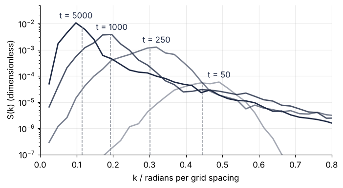
Structure factor S(k) against wavenumber k at t = 50, 250, 1000 and 5000. The peak moves to smaller k and grows as the domains coarsen; dashed ticks mark 2π/R for each time.

The peak moves to smaller k and rises as the domains coarsen, from k ≈ 0.5 at t = 50 to 0.1 at t = 5,000. The dashed lines at 2π/R stay close to each peak, which is what a domain size read from S should do.

Step 6: Fit the growth exponent and draw the coarsening

A power law R ∝ tⁿ is a straight line of slope n on log axes. Fit it over the last decade, t from 500 to 5,000, and over its two halves to see how much the slope moves:

def exponent(t1, t2, R=R_rec):
    sel = (t_rec >= t1 * 0.999) & (t_rec <= t2 * 1.001)
    return np.polyfit(np.log(t_rec[sel]), np.log(R[sel]), 1)[0]

t_mid = np.sqrt(500 * T)
n_fit = exponent(500, T)
print(f"n over [500, 5000]  = {n_fit:.3f}")
print(f"n over [500, {t_mid:.0f}] = {exponent(500, t_mid):.3f},  over [{t_mid:.0f}, 5000] = {exponent(t_mid, T):.3f}")
print(f"R(T) / L = {R_rec[-1] / L:.3f}")

n over [500, 5000]  = 0.313
n over [500, 1581] = 0.292,  over [1581, 5000] = 0.321
R(T) / L = 0.213

fig = plt.figure(figsize=(8, 4))
gs = fig.add_gridspec(2, 4, width_ratios=[1, 1, 0.45, 2.2], wspace=0.08, hspace=0.08)
for i, (t_snap, (c_snap, _)) in enumerate(snaps.items()):
    ax = fig.add_subplot(gs[i // 2, i % 2])
    im = ax.imshow(c_snap, cmap="cividis", vmin=-1, vmax=1, origin="lower")
    ax.set(xticks=[], yticks=[])
    ax.grid(False)
    ax.text(0.04, 0.95, f"t = {t_snap}", transform=ax.transAxes, va="top", color="white",
            bbox=dict(boxstyle="round,pad=0.2", fc=INK, ec="none", alpha=0.8))
cbar = fig.colorbar(im, ax=fig.axes, location="bottom", shrink=0.8, aspect=30, pad=0.04, ticks=[-1, 0, 1])
cbar.set_label("composition c")

ax = fig.add_subplot(gs[:, 3])
sel = t_rec >= 500 * 0.999                                  # the fit window, [500, T]
ax.loglog(t_rec, R_rec, "o", color=INK, ms=4)
coef = np.polyfit(np.log(t_rec[sel]), np.log(R_rec[sel]), 1)
ax.loglog(t_rec[sel], np.exp(np.polyval(coef, np.log(t_rec[sel]))), color=ACCENT, zorder=3)
ax.text(600, np.exp(np.polyval(coef, np.log(600))) * 0.74, f"fit: n = {n_fit:.2f}", color=ACCENT)
t_ref = t_rec[sel][0]
ax.loglog(t_rec, R_rec[sel][0] * (t_rec / t_ref)**(1 / 3), color=MUTED, ls="--", lw=1)
ax.text(25, R_rec[sel][0] * (25 / t_ref)**(1 / 3) * 0.8, "t$^{1/3}$", color=MUTED)
ax.set(xlabel="t (dimensionless)", ylabel="R / grid spacings")
ax.set_yticks([10, 20, 30, 40, 60], labels=["10", "20", "30", "40", "60"], minor=False)
ax.minorticks_off()
plt.show()

Left: the blend at t = 50, 250, 1000 and 5000, a fine labyrinth coarsening into wide domains. Right: domain size R against time on log axes; the fitted slope n = 0.31 runs just below the dashed t^1/3 line.

The exponent comes out at 0.31 against 1/3, with 0.29 on the first half of the decade and 0.32 on the second. It creeps up toward 1/3 from below, as Huse showed: at these times a correction that fades as the domains grow still pulls the slope down. The exponent names the mechanism: 1/3 for bulk diffusion between domains, 1/4 when material moves mainly along the interfaces, and something else again when c is not conserved (see Variations).

Pitfalls

Fitting over the early times. Fit the same data from t = 20 and the exponent drops from 0.31:

print(f"n over [20, 5000] = {exponent(20, T):.3f}")

n over [20, 5000] = 0.276

Before a few hundred time units the field is still separating: in the final figure R even shrinks until about t = 50, while the noise sorts itself into the fastest-growing wavelength of Step 2, about 13. Neither that stage nor the crossover after it is a power law, and a fit that starts there mixes them into a number that belongs to nothing. The early fit gives 0.28. Fit the last decade, and keep R well below L, where the periodic box does not yet shape the domains; Step 6 ends at a fifth of L.

A time step past 2κ. Past the bound of Step 3 the run does not explode. It flickers. Continue Step 5's run from t = 1,000 to t = 2,000, once at Δt = 2 and once at Δt = 5:

for dt in [2.0, 5.0]:
    ch_p = snaps[1000][1].copy()
    for _ in range(round(1000 / dt)):
        ch_prev, ch_p = ch_p, step(ch_p, dt=dt, keep=keep)
    change = w * np.abs(ch_p - ch_prev)**2
    k2_flip = k2.flat[change.argmax()]                        # the mode that changed most in the last step
    jump = np.abs(irfft2(ch_p - ch_prev, s=(N, N))).max()
    print(f"dt = {dt:.0f}: R = {domain_size(ch_p):.1f}, max |c| = {np.abs(irfft2(ch_p, s=(N, N))).max():.2f}, "
          f"last step moves c by up to {jump:.2f}, mostly at k² = {k2_flip:.2f}")

dt = 2: R = 40.7, max |c| = 1.03, last step moves c by up to 0.01, mostly at k² = 0.02
dt = 5: R = 40.2, max |c| = 1.21, last step moves c by up to 0.53, mostly at k² = 0.42

At Δt = 5 the field overshoots to 1.21, and the last step alone moves it by half a unit, mostly in modes near k² = 1/κ = 0.5, the worst case of Step 3. R differs from the honest run by about 1 % and looks fine. Watch max |c| and the change per step, not R, and confirm any new Δt with a run at half the step.

Measuring R from the peak or the mean wavenumber. The peak of S sits on rings 2π/L ≈ 0.025 apart, so at late times its position jumps between a handful of rings and the fit with it. The common alternative, 2π over the mean wavenumber, is pulled down by the large-k tail that sharp interfaces put into S, and it gives a lower exponent on the same run:

print(f"n from 2π/<k> over [500, 5000] = {exponent(500, T, R=2 * np.pi / k1_rec):.3f}, from the mean wavelength {n_fit:.3f}")

n from 2π/<k> over [500, 5000] = 0.261, from the mean wavelength 0.313

It gives 0.26 against 0.31. The mean wavelength of Step 1 weights each mode by 1/|k| instead and is not dominated by the interfaces.

Variations

Droplets instead of a labyrinth. Start from c = 0.4 plus noise. A mixture is unstable to any small fluctuation where the slope of c³ − c, 3c² − 1, is negative, which is for |c| < 1/√3 ≈ 0.58, the spinodal. At 0.4 the minority phase takes 30 % of the area, by the lever rule, and forms round droplets. Lifshitz and Slyozov solved the dilute limit of this case, in three dimensions: their t^⅓ carries over to this fraction, their solution for the droplet sizes does not.
Non-conserved ordering (Allen-Cahn). Drop the outer k² everywhere, so that the update becomes \((\hat c - \Delta t\,\mathcal F[c^3 - c])/(1 + \Delta t\,\kappa k^2)\). Now c is no longer conserved, domains shrink by their own curvature, and R grows as t^½.
A larger step. Add \(A k^2\hat c\) to both sides of the update, implicitly on the left and explicitly on the right. This is the stabilized scheme, which buys steps beyond 2κ at some cost in early-time accuracy.
Three dimensions. rfftn and irfftn on a 128³ grid with the same mask on all three axes.

Cheat sheet

kx = 2 * np.pi * fftfreq(N, d=dx)                         # axis 0: all wavenumbers, radians
ky = 2 * np.pi * rfftfreq(N, d=dx)                        # axis 1: nonnegative half
KX, KY = np.meshgrid(kx, ky, indexing="ij"); k2 = KX**2 + KY**2
keep = (abs(KX) < np.pi / dx / 2) & (abs(KY) < np.pi / dx / 2)   # 1/2 rule for a cubic term
c = irfft2(ch, s=(N, N))                                  # s= or the shape is guessed
ch = (ch - dt * k2 * keep * rfft2(c**3 - c)) / (1 + dt * kappa * k2**2)   # stable for dt <= 2 * kappa
kinv = np.divide(1, np.sqrt(k2), out=np.zeros_like(k2), where=k2 > 0)        # 1/|k|, 0 at k = 0
w = np.full(k2.shape, 2.0); w[:, 0] = w[:, -1] = 1; w[0, 0] = 0              # mirrored columns twice, no mean
S = w * abs(ch)**2; R = 2 * np.pi * (S * kinv).sum() / S.sum()                # domain size, the mean wavelength
# stiff constant-coefficient part implicit (a division), cube explicit; check with half the step