Fixation probability by simulation: how often a beneficial mutation survives

The problem

You know the size of a population and the selective advantage of a new mutation, and you want its fixation probability, the chance that a single new copy takes over, with an error bar and a check against theory. The example is a Wright-Fisher population of N = 100 diploid individuals, 200 gene copies, one of them a mutation with s = 0.01. Selection weights its frequency \(p\) first: each copy counts \(1 + s\) times, divided by the mean fitness \(1 + ps\), so genotypes with zero, one, and two copies have fitnesses 1, \(1 + s\), and \((1 + s)^2 \approx 1 + 2s\). Then a binomial draw from a seeded generator picks the next 200 copies, as in genetic drift. Swap in your own N, s, and starting count.

The code

Copy

import numpy as np
import matplotlib.pyplot as plt

# ---- population and mutation: replace with your own
N = 100                                    # diploid individuals, so 2N gene copies
TWO_N = 2 * N
k0 = 1                                     # copies of the mutation at the start
s_values = np.array([0, 0.0025, 0.005, 0.01, 0.015, 0.02, 0.03, 0.04])
R = 50_000                                 # populations per value of s
rng = np.random.default_rng(310)

# ---- selection, then drift, until every population is decided
def fixation(s):
    k = np.full(R, k0)
    open_ = np.arange(R)                   # only these are drawn again
    while open_.size:
        p = k[open_] / TWO_N
        p_sel = p * (1 + s) / (1 + p * s)
        k[open_] = rng.binomial(TWO_N, p_sel)
        open_ = open_[(k[open_] > 0) & (k[open_] < TWO_N)]
    return np.mean(k == TWO_N)

# ---- theory: Kimura's formula for a start at frequency p0
def kimura(s, p0=k0 / TWO_N):
    s = np.atleast_1d(np.asarray(s, dtype=float))
    u = np.full(s.shape, p0)               # the neutral limit, used at s = 0
    x = -4 * N * s[s != 0]
    u[s != 0] = np.expm1(x * p0) / np.expm1(x)   # exp(x) - 1
    return u

# ---- estimate with error bars
u = np.array([fixation(s) for s in s_values])
se = np.sqrt(u * (1 - u) / R)
theory = kimura(s_values)

# ---- report and plot
print("     s     simulated u    Kimura     2s   distance")
for s, ui, sei, th in zip(s_values, u, se, theory):
    print(f"{s:6.4f}  {ui:.4f} ± {sei:.4f}  {th:.4f}  {2 * s:.3f}  {(ui - th) / sei:+5.1f} se")

s_fine = np.linspace(0, 0.042, 300)
fig, (ax, ax2) = plt.subplots(2, 1, sharex=True, figsize=(7, 4.4), dpi=110)
ax.plot(s_fine, kimura(s_fine), color="#1f2a44", lw=1.8)
ax.plot(s_fine, 2 * s_fine, color="#8a8f98", lw=1, ls="--")
ax.axhline(1 / TWO_N, color="#2a7f9e", lw=1, ls="--")
ax.errorbar(s_values, u, yerr=2 * se, fmt="o", color="#c8553d", ms=4, capsize=2, lw=1, zorder=3)
ax.text(0.034, 0.054, "Kimura", color="#1f2a44")
ax.text(0.0325, 0.073, "2s", color="#8a8f98", ha="right")
ax.text(0.041, 0.008, "1/2N", color="#2a7f9e", ha="right")
ax.text(0.0165, 0.040, "simulated ± 2 se", color="#c8553d", ha="right")
ax.set(ylabel="fixation probability", ylim=(0, 0.088))
ax2.axhline(0, color="#1f2a44", lw=1.2)          # Kimura's value, the reference
ax2.errorbar(s_values, (u - theory) / se, yerr=2, fmt="o", color="#c8553d", ms=4, capsize=2, lw=1)
ax2.set(xlabel="selective advantage per copy, s", ylabel="distance / se",
        xlim=(-0.001, 0.042), ylim=(-4.5, 4.5))
for a in (ax, ax2): a.spines[["top", "right"]].set_visible(False)
plt.show()

     s     simulated u    Kimura     2s   distance
0.0000  0.0047 ± 0.0003  0.0050  0.000   -1.0 se
0.0025  0.0076 ± 0.0004  0.0079  0.005   -0.9 se
0.0050  0.0109 ± 0.0005  0.0115  0.010   -1.3 se
0.0100  0.0194 ± 0.0006  0.0202  0.020   -1.2 se
0.0150  0.0284 ± 0.0007  0.0296  0.030   -1.7 se
0.0200  0.0397 ± 0.0009  0.0392  0.040   +0.5 se
0.0300  0.0575 ± 0.0010  0.0582  0.060   -0.7 se
0.0400  0.0778 ± 0.0012  0.0769  0.080   +0.7 se

The knobs

s and N act together. The theory line is Kimura's formula for a mutation that starts at frequency \(p_0 = k_0/2N\):

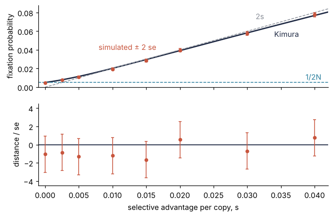
For one new copy, \(p_0 = 1/2N\), the numerator is \(1 - e^{-2s} \approx 2s\), so in units of the neutral 1/2N the fixation probability depends on s and N only through 4Ns: \(2N u \approx 4Ns / (1 - e^{-4Ns})\). At 4Ns = 4, the s = 0.01 row, the mutation fixes about four times as often as a neutral one, 0.0202 against 0.0050, close to Haldane's 2s = 0.020, the limit for 4Ns well above 1. For 4Ns well below 1 the curve flattens onto 1/2N and selection vanishes in drift: the leftmost points of the upper panel. R sets the error bar. The fixation probability is a mean of zeros and ones, so its standard error is \(\sqrt{u(1 - u)/R}\), 3.2 % of u at s = 0.01, as in the Monte Carlo failure probability recipe, and halving it takes four times the populations. k0 turns a new mutation into standing variation, and kimura follows it through \(p_0\).

The code simulates a Wright-Fisher population of constant size, with fitness per copy as in The problem and no new mutation along the way; its N is the effective size \(N_e\) of the drift tutorial. Kimura's formula approximates that model: it lets the frequency change smoothly instead of in steps of 1/2N, which is accurate for large N and small s (the diffusion approximation). The exact Wright-Fisher value, computed from the model's 201 possible copy numbers, lies 0.4 % below Kimura's at s = 0.01, far inside the 3.2 % error bar, so agreement says the code is right. The ± is sampling error only. The last column, plotted in the lower panel, gives each point's distance from Kimura in standard errors. Within about 2 is agreement, and one point in twenty lands beyond 2 by chance; several, or one at 4, mean a bug or a mismatch of conventions. Most beneficial mutations are lost, 98 in 100 here, because a single copy leaves no descendants in the next draw with probability 0.37, and an advantage of 1 % barely changes that, to 0.36. Selection takes hold once drift has carried the mutation to a few dozen copies: from 50 copies Kimura's formula gives 0.64, against 0.25 without selection. A branching process describes why the first copies decide.

Pitfalls

Stopping after a fixed number of generations. A loop of 200 generations looks generous for 200 copies. In a fresh run at s = 0.01 it leaves 0.37 % of the populations fixed and 2.4 % still carrying the mutation, against 1.98 % fixed at the end: counting the fixed underestimates u by a factor of five, and counting the not-lost overestimates it. The mutations that do fix take 335 generations on average, and the slowest population of that run was decided only after 1,474. Run until every population is decided, as the while loop does. Drawing only the open populations makes the long tail cheap, since most drop out in the first few generations.

A factor of two in s. The simulation sits at about twice or half the theory curve, and the distance column shows double-digit standard errors. Textbooks write s in two ways. This recipe's s is the advantage per copy, with the genotype fitnesses of The problem. A textbook that writes 1, 1 + s/2, 1 + s for zero, one, and two copies (additive selection, also written 1 + hs with h = 1/2) gives the whole s to the homozygote, so its advantage per copy is s/2 and its fixation probability is about s rather than 2s. Kimura's formula with s/2 gives 0.0115 here instead of 0.0202, 13 standard errors from the simulation. Halve the textbook's s in the additive case and put that same value into both the simulation and the formula. With dominance, h other than 1/2, no single per-copy s describes the three genotypes, and this recipe does not cover it.

Kimura's formula at s = 0. Written for one copy as (1 - np.exp(-2*s)) / (1 - np.exp(-4*N*s)), the formula returns nan and a RuntimeWarning in the s = 0 row. It is 0/0 there, though the limit is plain: 1/2N for one copy, k0/2N in general. Code the limit, as kimura does, and use np.expm1, which keeps the digits that \(1 - e^{-x}\) loses for tiny \(x\). At \(s = 10^{-12}\) the plain version is already wrong in the fifth digit.