Branching processes: why one neutron rarely starts a lasting fission chain (Python)

The question

A research reactor is brought to k = 1.001 with no neutron source inside: on average, 1,000 neutrons in one generation make 1,001 in the next. One stray neutron starts a chain. It causes a fission with probability p = 0.4120, and otherwise it is captured or leaks out. A fission yields ν neutrons. Most are released at the moment of fission, 0 to 7 of them, with the measured distribution for uranium-235 split by a slow neutron. With probability 0.0158 a delayed neutron follows, released a fraction of a second to about a minute later by a decaying fission fragment. That makes ν̄ = 2.430 neutrons per fission on average, and k = p ν̄ counts both kinds. Whether the chain lasts is a question about a branching process. Here are 40 such chains and the first lasting one among 10,000:

Show code

import numpy as np
import matplotlib.pyplot as plt

plt.rcParams.update({
    "figure.figsize": (7, 3.6), "figure.dpi": 110,
    "axes.spines.top": False, "axes.spines.right": False,
    "axes.grid": True, "grid.alpha": 0.25,
    "font.size": 11, "lines.linewidth": 1.8,
})
INK, ACCENT, SECOND, MUTED = "#1f2a44", "#c8553d", "#2a7f9e", "#8a8f98"

# Neutrons released at the moment of a thermal fission of U-235, nu = 0..7, from N. E. Holden and
# M. S. Zucker, BNL-NCS-35513 (1985), https://www.osti.gov/servlets/purl/6205262.
# The eight numbers sum to 1.0000003, so they are normalized.
P_AT_ONCE = np.array([0.0317223, 0.1717071, 0.3361991, 0.3039695, 0.1269459, 0.0266793, 0.0026322, 0.0001449])
P_AT_ONCE /= P_AT_ONCE.sum()
NU_DELAYED = 0.0158                          # delayed neutrons per fission; never more than one counted
P_NU = (1 - NU_DELAYED) * np.append(P_AT_ONCE, 0) + NU_DELAYED * np.append(0, P_AT_ONCE)
NU = np.arange(P_NU.size)                    # 0..8 neutrons per fission
nu_bar = P_NU @ NU
D = P_NU @ (NU * (NU - 1)) / nu_bar**2       # Diven factor: the spread of nu that matters here
print(f"neutrons per fission: released at once {P_AT_ONCE @ np.arange(8):.3f}, in all {nu_bar:.3f};  D = {D:.3f}")


def offspring_pmf(k, P=P_NU):
    """P(X = j), the children of one neutron: no fission with chance 1 - p, else nu children from P."""
    p = k / (P @ np.arange(P.size))
    pmf = p * P
    pmf[0] += 1 - p
    return pmf


# The chains are simulated by the method this tutorial explains, so that the answer
# can be checked at the end. Pretend you have not seen this cell.
rng = np.random.default_rng(20261010)


def simulate(k, n_chains, cap=10_000, record=False):
    """Chains of one neutron each, run until every chain is dead or has reached cap neutrons."""
    pmf = offspring_pmf(k)
    children = np.arange(pmf.size)
    Z = np.ones(n_chains, dtype=np.int64)
    death = np.zeros(n_chains, dtype=int)    # generation in which the chain died, 0 if it lasted
    lasting = np.zeros(n_chains, dtype=bool)
    alive = np.arange(n_chains)
    log, n = [], 0
    while alive.size:
        n += 1
        # sort the Z neutrons of each chain by their number of children, then add the children up
        Z_new = rng.multinomial(Z[alive], pmf) @ children
        if record:
            log.append((alive, Z_new))
        Z[alive] = Z_new
        death[alive[Z_new == 0]] = n
        lasting[alive[Z_new >= cap]] = True
        alive = alive[(Z_new > 0) & (Z_new < cap)]
    assert np.all(lasting != (death > 0))    # every chain decided, one way or the other
    return death, lasting, log


def path(log, i):
    """Neutron numbers of chain i, generation by generation, from a recorded run."""
    Z = [1]
    for alive, Z_new in log:
        j = np.searchsorted(alive, i)
        if j == alive.size or alive[j] != i:
            break
        Z.append(Z_new[j])
    return np.array(Z)


K_REACTOR = 1.001
death, lasting, log = simulate(K_REACTOR, 10_000, record=True)
dead = death > 0
print(f"dead after generation 1: {np.mean(death == 1):.1%},  by generation 10: {np.mean(dead & (death <= 10)):.1%}")
print(f"dead chains: median lifetime {np.median(death[dead]):.0f} generation, longest {death.max():,} generations")
print(f"lasting (reached 10,000 neutrons): {lasting.sum()} of {death.size:,};  among the first 40: {lasting[:40].sum()}")

paths = [path(log, i) for i in range(40)]
first_lasting = path(log, np.flatnonzero(lasting)[0])
print(f"the first lasting chain passes 10,000 neutrons in generation {first_lasting.size - 1:,}, "
      f"where the mean is 1.001ⁿ = {K_REACTOR ** (first_lasting.size - 1):.2f}")
fig, ax = plt.subplots(figsize=(8, 3.6))
for Z in paths:
    ax.step(np.arange(Z.size), Z, where="post", color=MUTED, lw=1, alpha=0.7)
    ax.plot(Z.size - 1, 0, "o", ms=4, color=MUTED, clip_on=False)
ax.step(np.arange(first_lasting.size), first_lasting, where="post", color=ACCENT, lw=1.4)
n = np.arange(first_lasting.size)
ax.plot(n, K_REACTOR**n, color=SECOND, lw=1.2, ls="--")
ax.text(first_lasting.size - 1, 1.6 * K_REACTOR ** n[-1], "mean 1.001ⁿ", color=SECOND, ha="right", va="bottom")
ax.text(300, 250, "a lasting chain", color=ACCENT, ha="center", va="top")
ax.text(0.05, 3000, f"{100 * np.mean(death == 1):.1f} % of 10,000 chains\nare dead after one generation", color=INK, va="center")
ax.set_xscale("symlog", linthresh=1, linscale=0.4)            # room for the first generations, zero included
ax.set_yscale("symlog", linthresh=1, linscale=0.4)            # zero gets a row of its own
ax.minorticks_off()
ticks = [0, 1, 2, 5, 10, 20, 50, 100, 200, 500, 1000]
ax.set(xlim=(0, first_lasting.size), ylim=(0, 2e4), xticks=ticks, xticklabels=[f"{t:,}" for t in ticks],
       yticks=[0, 1, 10, 100, 1000, 10_000], yticklabels=["0", "1", "10", "100", "1,000", "10,000"],
       xlabel="generation n", ylabel="neutrons Zₙ")
plt.show()

neutrons per fission: released at once 2.414, in all 2.430;  D = 0.799
dead after generation 1: 60.6%,  by generation 10: 91.8%
dead chains: median lifetime 1 generation, longest 2,384 generations
lasting (reached 10,000 neutrons): 9 of 10,000;  among the first 40: 0
the first lasting chain passes 10,000 neutrons in generation 1,378, where the mean is 1.001ⁿ = 3.96

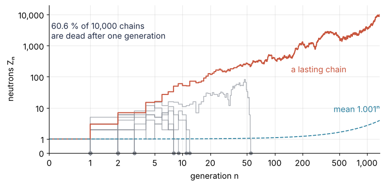
Neutron number against generation for 40 chains of one neutron at k = 1.001, both axes logarithmic, zero included. All 40 die within 55 generations, most in the first. The first lasting chain of 10,000 climbs above the mean 1.001ⁿ and reaches 10,000 neutrons at generation 1,378.

Of the 10,000 chains, 60.6 % are dead after one generation and 91.8 % by generation 10, and the median dead chain lived for a single generation. The mean, 1.001ⁿ, is still below 4 at generation 1,378, where the lasting chain passes 10,000 neutrons. That is where the simulation calls a chain lasting, because from there its chance of still dying is negligible; the number comes at the end. Nine chains of 10,000 got there. The longest-lived chain that did die held on for 2,384 generations.

The mean says the neutron population grows, and still most chains die at once. The question is what fraction of single neutrons starts a chain that never dies, and how that fraction depends on k and on the spread of ν. The answer also explains why a reactor startup insists on a neutron source when in principle one neutron is enough.

The idea: a chain dies only if every branch dies

Follow one neutron. Either it causes no fission, with probability 1 − p, or it causes one and has ν children drawn from P(ν). Every neutron does this independently, with the same odds, whatever happened to its ancestors and siblings. A chain built this way is a Galton-Watson branching process, and the number of children X of one neutron is its offspring distribution:

Show code

pmf_X = offspring_pmf(K_REACTOR)
print(f"P(X = 0) = {pmf_X[0]:.3f},  mean of X = {pmf_X @ NU:.4f}")
print(f"simulated share of chains dead after one generation {np.mean(death == 1):.3f}")

fig, (ax1, ax2) = plt.subplots(2, 1, figsize=(7, 4.4), sharex=True)
ax1.bar(NU, P_NU, width=0.7, color=INK)
ax1.axvline(nu_bar, color=MUTED, lw=1, ls="--")
ax1.text(nu_bar + 0.12, 0.37, f"mean ν̄ = {nu_bar:.3f}", color=MUTED, va="center")
ax1.set(ylabel="P(ν)", ylim=(0, 0.4))
ax2.bar(NU, pmf_X, width=0.7, color=ACCENT)
ax2.text(0.42, pmf_X[0], f"{pmf_X[0]:.3f}", color=ACCENT, va="center")
ax2.set(ylabel="P(X)", xlabel="neutrons per fission ν (top), children of one neutron X (bottom)",
        xticks=NU, ylim=(0, 0.7))
plt.show()

P(X = 0) = 0.601,  mean of X = 1.0010
simulated share of chains dead after one generation 0.606

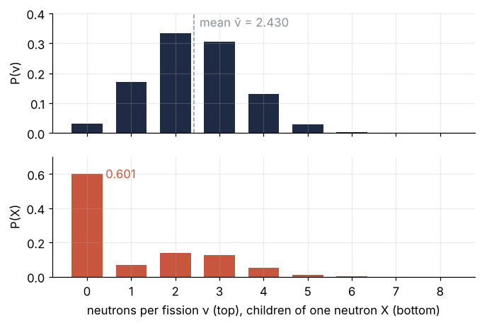
Top: probability of ν neutrons per uranium-235 fission, delayed neutron included, ν = 0 to 8, mean 2.430. Bottom: probability of X children of one neutron at k = 1.001; the zero bar, 0.601, dominates.

The chance of no children at all is P(X = 0) = 1 − p + p P(ν = 0) = 0.601, which is the first-generation death share of the question seen from the other side. The mean of X is k = 1.001.

A chain started by one neutron dies if and only if each of the chains started by its children dies. Those subchains are independent, and each is a copy of the whole problem: one neutron, the same odds. So if q is the probability that a chain dies, a neutron with j children has a line that dies with probability \(q^j\), and summing over j,

\[q = \sum_j P(X = j)\, q^j .\]

The right side is a power series in q. Write it with a free variable s and it gets its name, the generating function of X:

\[f(s) = \sum_j P(X = j)\, s^j = \langle s^X \rangle ,\]

with ⟨·⟩ the average over X. For fission, by the same two cases as above, f(s) = 1 − p + p g(s), where \(g(s) = \sum_\nu P(\nu)\, s^\nu\) is the generating function of the fission itself. The extinction probability q is a point where the curve f(s) meets the diagonal. Here it is at three values of k:

Show code

def f(s, pmf):
    return np.polynomial.polynomial.polyval(s, pmf)


s = np.linspace(0, 1, 300)
fig, ax = plt.subplots(figsize=(7, 4))
ax.plot(s, s, color=MUTED, lw=1, ls="--")
for k, alpha in [(0.8, 0.35), (1.0, 0.65), (1.3, 1.0)]:
    ax.plot(s, f(s, offspring_pmf(k)), color=INK, alpha=alpha)
    ax.text(0.02, f(0, offspring_pmf(k)) + 0.025, f"k = {k}", color=INK, alpha=alpha, va="bottom")
q = 0.0
for _ in range(500):                     # q_n = f(q_(n-1)) from q_0 = 0, as explained below
    q = f(q, offspring_pmf(1.3))
ax.plot([q, 1], [q, 1], "o", ms=6, color=ACCENT)
ax.text(q + 0.02, q - 0.04, f"q = {q:.3f}", color=ACCENT, va="top")
ax.set(xlabel="s", ylabel="f(s)", xlim=(0, 1.02), ylim=(0, 1.02))
plt.show()

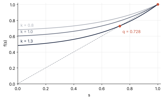
Generating function f(s) against s for k = 0.8, 1.0 and 1.3, with the diagonal. All three end at f(1) = 1; only for k = 1.3 does the curve cross the diagonal below 1, at q = 0.728.

Every curve ends at f(1) = 1, because the probabilities add up to one, so s = 1 always solves f(s) = s. The slope there is f′(1) = Σ j P(X = j) = k. All coefficients of f are nonnegative, so f bends upward and meets a straight line at most twice. For k = 0.8 and 1.0 the curve stays above the diagonal and meets it only at 1. For k = 1.3 it arrives at 1 steeper than the diagonal, so it must have crossed it once before, at q = 0.728.

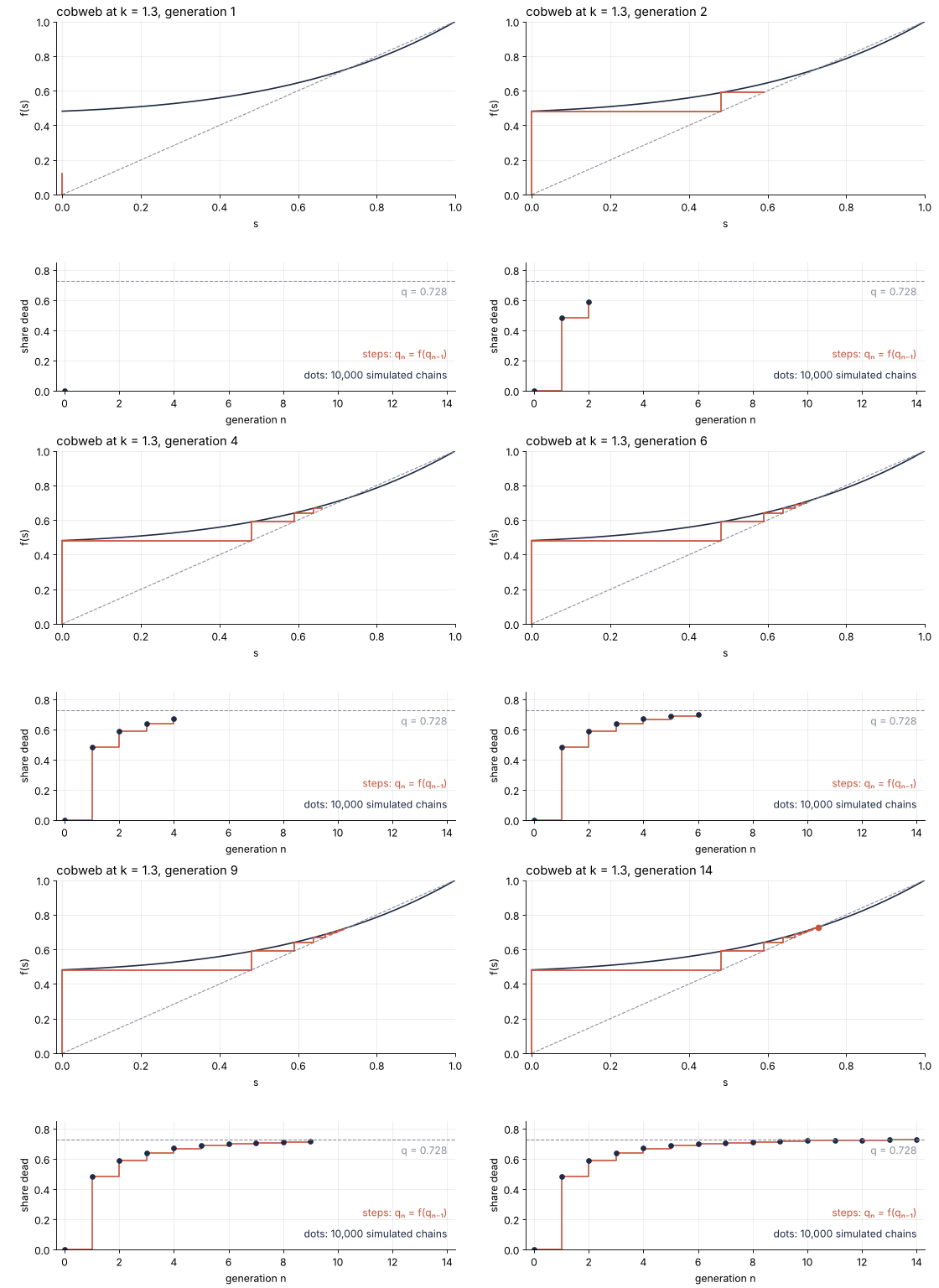
Of the two roots, the chain takes the smaller. Let \(q_n\) be the probability that the chain is dead by generation n. It is dead by then exactly when every child's subchain is dead within the n − 1 generations left to it, so \(q_n = f(q_{n-1})\), starting from \(q_0 = 0\), since one neutron is alive at generation 0. Because f increases, a value below q is mapped to a value below q: the sequence climbs, stops at the smaller root, and never reaches 1. A cobweb draws this iteration. From the diagonal go up to the curve, across to the diagonal, and repeat:

Top: the cobweb of q_n = f(q_(n-1)) at k = 1.3 grows step by step from 0 toward the crossing at 0.728. Bottom: the predicted q_n as steps and the share of 10,000 simulated chains dead by generation n as dots; they agree at every step and level off near 0.728.

Show code

"""Extinction cobweb: the iteration q_n = f(q_(n-1)) at k = 1.3, against simulated chains.

Renders ../../assets/extinction-cobweb.gif. Top: the generating function f(s) of the children
of one neutron, the diagonal, and the cobweb from q_0 = 0, one segment at a time. Bottom: q_n
against generation n, the predicted steps and the share of 10,000 simulated chains dead by
generation n. Run it from any directory:

    python scene.py
"""
from pathlib import Path

import matplotlib
import numpy as np

matplotlib.use("Agg")
import matplotlib.pyplot as plt
from matplotlib.animation import FuncAnimation, PillowWriter
from PIL import Image

OUT = Path(__file__).resolve().parents[2] / "assets" / "extinction-cobweb.gif"
INK, ACCENT, SECOND, MUTED = "#1f2a44", "#c8553d", "#2a7f9e", "#8a8f98"
plt.rcParams.update({"axes.spines.top": False, "axes.spines.right": False,
                     "axes.grid": True, "grid.alpha": 0.25, "font.size": 11})

# ---- the model of the tutorial: neutrons per fission of U-235, one delayed neutron with chance 0.0158
P_AT_ONCE = np.array([0.0317223, 0.1717071, 0.3361991, 0.3039695, 0.1269459, 0.0266793, 0.0026322, 0.0001449])
P_AT_ONCE /= P_AT_ONCE.sum()
P_NU = (1 - 0.0158) * np.append(P_AT_ONCE, 0) + 0.0158 * np.append(0, P_AT_ONCE)
NU = np.arange(P_NU.size)
K, N_CHAINS, N_GEN = 1.3, 10_000, 14

p = K / (P_NU @ NU)
pmf = p * P_NU
pmf[0] += 1 - p


def f(s):
    return np.polynomial.polynomial.polyval(s, pmf)


q = [0.0]
for n in range(N_GEN):
    q.append(f(q[-1]))
q = np.array(q)
q_root = q[-1]
for _ in range(500):                                         # the fixed point itself, for the guide line
    q_root = f(q_root)

# ---- the simulated share dead by generation n, with its own generator
rng = np.random.default_rng(20261011)
Z = np.ones(N_CHAINS, dtype=np.int64)
dead = [0.0]
for n in range(N_GEN):
    alive = (Z > 0) & (Z < 10_000)                          # a chain at 10,000 neutrons counts as lasting
    Z[alive] = rng.multinomial(Z[alive], pmf) @ NU
    dead.append(np.mean(Z == 0))

# ---- frames: per generation, three frames up to the curve, three across to the diagonal
FRAMES_PER_HALF, HOLD = 4, 18
frames = [(n, part, i) for n in range(1, N_GEN + 1) for part in (0, 1) for i in range(1, FRAMES_PER_HALF + 1)]
frames += [frames[-1]] * HOLD

fig, (ax1, ax2) = plt.subplots(2, 1, figsize=(7, 6.4), dpi=80, height_ratios=[1.35, 1])
fig.subplots_adjust(left=0.12, right=0.97, top=0.95, bottom=0.09, hspace=0.45)
s = np.linspace(0, 1, 300)


def update(frame):
    n_now, part, i = frame
    ax1.clear(); ax2.clear()
    ax1.plot(s, f(s), color=INK)
    ax1.plot(s, s, color=MUTED, lw=1, ls="--")
    # the cobweb up to the current segment: up from (q_{n-1}, q_{n-1}) to the curve, across to the diagonal
    xs, ys = [0.0], [0.0]
    for n in range(1, n_now + 1):
        x0, y1 = q[n - 1], q[n]
        if n < n_now:
            xs += [x0, y1]; ys += [y1, y1]
        else:
            t = i / FRAMES_PER_HALF
            if part == 0:
                xs.append(x0); ys.append(x0 + t * (y1 - x0))
            else:
                xs += [x0, x0 + t * (y1 - x0)]; ys += [y1, y1]
    ax1.plot(xs, ys, color=ACCENT, lw=1.6)
    ax1.plot(q_root, q_root, "o", ms=6, color=ACCENT, alpha=1.0 if n_now == N_GEN and part == 1 else 0.0)
    ax1.set(xlim=(-0.015, 1), ylim=(0, 1), xlabel="s", ylabel="f(s)")   # the first step runs up s = 0, off the spine
    ax1.set_title(f"cobweb at k = {K}, generation {n_now}", loc="left")

    shown = n_now if part == 1 else n_now - 1
    gens = np.arange(shown + 1)
    ax2.step(gens, q[: shown + 1], where="post", color=ACCENT)
    ax2.plot(gens, dead[: shown + 1], "o", ms=5, color=INK)
    ax2.axhline(q_root, color=MUTED, lw=1, ls="--")
    ax2.text(N_GEN, q_root - 0.03, f"q = {q_root:.3f}", color=MUTED, ha="right", va="top")
    ax2.set(xlim=(-0.3, N_GEN + 0.3), ylim=(0, 0.85), xlabel="generation n", ylabel="share dead")
    ax2.text(N_GEN, 0.22, "steps: qₙ = f(qₙ₋₁)", color=ACCENT, ha="right")
    ax2.text(N_GEN, 0.08, "dots: 10,000 simulated chains", color=INK, ha="right")


OUT.parent.mkdir(exist_ok=True)
FuncAnimation(fig, update, frames=frames).save(OUT, writer=PillowWriter(fps=12))
plt.close(fig)
print(f"q_n: {', '.join(f'{x:.3f}' for x in q)}")
print(f"simulated: {', '.join(f'{x:.3f}' for x in dead)}")
with Image.open(OUT) as im:
    print(f"{OUT.name}: {im.width} x {im.height} px, {im.n_frames} frames, {OUT.stat().st_size / 1024:,.0f} kB")

The dots of the simulation sit on every step.

Just above critical: why the chance grows as k − 1

At k = 1.001 the second crossing is a hair below 1, and the shape of f near s = 1 decides where it is. Expand f to second order in 1 − s,

\[f(s) \approx 1 - k\,(1 - s) + \tfrac{1}{2} f''(1)\,(1 - s)^2 ,\]

with f′(1) = k and f″(1) = ⟨X(X − 1)⟩, both read off by differentiating the power series at s = 1. Setting f(s) = s and dividing by 1 − s gives the survival probability π = 1 − q:

\[\pi \approx \frac{2\,(k - 1)}{f''(1)} .\]

A slope greater than 1 pushes the crossing away from 1, and the curvature pulls it back. From f(s) = 1 − p + p g(s), f″(1) = p ⟨ν(ν − 1)⟩. With p = k/ν̄ and the Diven factor D = ⟨ν(ν − 1)⟩/ν̄², which measures the spread of ν (1 for a Poisson-distributed ν, 0.799 for the measured one), the curvature is f″(1) = k ν̄ D = 1.001 × 2.430 × 0.799 = 1.94, and π = 1.03 × 10⁻³. One neutron in 971 starts a lasting chain.

Iterating q = f(q) this close to critical takes about 10,000 steps to settle the fourth digit. Faster: divide the polynomial f(s) − s by s − 1 and take the smallest root in [0, 1) of the rest. The division matters: a root finder returns the root at 1 only to rounding, sometimes just below 1, and below critical it would then pass for q:

Show code

from numpy.polynomial import Polynomial


def extinction_q(pmf):
    """Smallest root of f(s) = s in [0, 1], with the root at s = 1 divided out first."""
    g, _ = divmod(Polynomial(pmf) - Polynomial([0, 1]), Polynomial([-1, 1]))
    roots = g.roots()
    real = roots[np.abs(roots.imag) < 1e-12].real
    inside = real[(real >= 0) & (real < 1)]
    return inside.min() if inside.size else 1.0


q_root = extinction_q(pmf_X)
q = 0.0
for _ in range(10_000):
    q = f(q, pmf_X)
f2 = pmf_X @ (NU * (NU - 1))
print(f"k = {K_REACTOR}:  pi from the root {1 - q_root:.4e},  after 10,000 steps of q = f(q) {1 - q:.4e}")
print(f"f''(1) = {f2:.3f},  linear law 2(k - 1)/f''(1) = {2 * (K_REACTOR - 1) / f2:.4e},  one in {1 / (1 - q_root):.0f}")
print(f"sibling pairs from X = 3 alone {6 * pmf_X[3]:.2f};  children per neutron that has any {K_REACTOR / (1 - pmf_X[0]):.2f};"
      f"  Poisson-distributed X with mean k: f''(1) = k² = {K_REACTOR**2:.2f}")

s = np.linspace(0.995, 1, 300)
u = 1 - s
fig, ax = plt.subplots()
ax.axhline(0, color=MUTED, lw=1)
ax.plot(s, 1e6 * (f(s, pmf_X) - s), color=INK)
ax.plot(s, 1e6 * (-(K_REACTOR - 1) * u + f2 / 2 * u**2), color=SECOND, lw=1.2, ls="--")
ax.plot(q_root, 0, "o", ms=6, color=ACCENT)
ax.annotate(f"q = {q_root:.5f}", (q_root, 0), xytext=(q_root - 0.0006, 5),
            color=ACCENT, ha="center", arrowprops=dict(arrowstyle="->", color=ACCENT, lw=1))
ax.text(0.9968, 15, "f(s) − s", color=INK)
ax.text(0.9968, 13.2, "second-order expansion (dashed)", color=SECOND)
ax.set(xlabel="s", ylabel="f(s) − s  / 10⁻⁶", xlim=(0.995, 1))
plt.show()

k = 1.001:  pi from the root 1.0303e-03,  after 10,000 steps of q = f(q) 1.0303e-03
f''(1) = 1.942,  linear law 2(k - 1)/f''(1) = 1.0298e-03,  one in 971
sibling pairs from X = 3 alone 0.75;  children per neutron that has any 2.51;  Poisson-distributed X with mean k: f''(1) = k² = 1.00

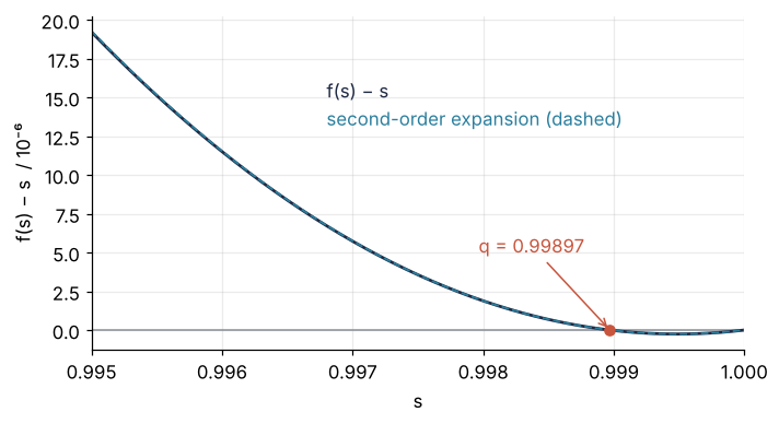
f(s) − s for s from 0.995 to 1 at k = 1.001, in units of 10⁻⁶, with its second-order expansion. The curve crosses zero 1.03 × 10⁻³ below 1, where the expansion crosses too.

Root and iteration agree in every printed digit, and the linear law is 0.05 % off.

Why is f″(1) as large as 1.94? ⟨X(X − 1)⟩ counts ordered pairs of siblings: a childless neutron adds none, and fissions with three neutrons alone add 0.75. The mean of X is held at k ≈ 1, so when three neutrons in five have no children, the others must make up for them: a neutron that has any children has 2.51 on average. Children come in bursts, and bursts make sibling pairs. A Poisson-distributed X with the same mean has f″(1) = k² = 1.00, and the bursts nearly halve the survival probability.

The spread of ν enters through D: at the same ν̄ and k, a narrower ν gives a smaller D, a flatter f, and a larger π. The measured ν is narrower than a Poisson-distributed ν, so the two comparisons point opposite ways. Compared with a Poisson-distributed X the real chain survives less often, compared with a Poisson-distributed ν more often:

Show code

import math

P_23 = np.zeros(9)
P_23[2], P_23[3] = 3 - nu_bar, nu_bar - 2                     # always 2 or 3, same mean
P_POISSON = np.array([math.exp(-nu_bar) * nu_bar**n / math.factorial(n) for n in range(31)])
P_POISSON /= P_POISSON.sum()
for name, P in [("nu always 2 or 3", P_23), ("measured P(nu)", P_NU), ("Poisson-distributed nu", P_POISSON)]:
    print(f"{name:24s} pi = {1 - extinction_q(offspring_pmf(K_REACTOR, P)):.3e}")

nu always 2 or 3         pi = 1.306e-03
measured P(nu)           pi = 1.030e-03
Poisson-distributed nu   pi = 8.228e-04

Two or three neutrons from every fission give 1.31 × 10⁻³, the measured ν 1.03 × 10⁻³, a Poisson-distributed ν 0.82 × 10⁻³.

Formalization

The chain starts with Z₀ = 1 neutron, and each generation is the sum of the children of the last,

\[Z_{n+1} = \sum_{i=1}^{Z_n} X_{n,i} ,\]

where the \(X_{n,i}\) are independent and all have the distribution P(X = j). Its generating function is the f(s) = \(\langle s^X \rangle\) = 1 − p + p g(s) of the idea section, with f(1) = 1, f′(1) = k and f″(1) = k ν̄ D. The generating function of \(Z_n\) is f applied n times, f(f(⋯f(s)⋯)), because each child of the first neutron starts its own chain with n − 1 generations to go. At s = 0 this gives back \(q_n = f(q_{n-1})\). The extinction probability q is the smallest root of f(s) = s in [0, 1], and the survival probability is π = 1 − q. The predictions for the example:

Show code

K_VALUES = [1.001, 1.003, 1.01, 1.03, 1.1, 1.3]
pi_root = {k: 1 - extinction_q(offspring_pmf(k)) for k in K_VALUES}
pi_law = {k: 2 * (k - 1) / (k * nu_bar * D) for k in K_VALUES}
print("    k       q        pi       2(k - 1)/(k nu D)   law / pi")
for k in K_VALUES:
    print(f"{k:6.3f}  {1 - pi_root[k]:.5f}  {pi_root[k]:.3e}   {pi_law[k]:.3e}          {pi_law[k] / pi_root[k]:.3f}")

print(f"\nmean neutrons in one chain at k = 0.99: 1/(1 - k) = {1 / (1 - 0.99):.0f}")
pi = pi_root[K_REACTOR]
for S in [10, 1e6]:
    print(f"source of {S:9,.0f} n/s at k = {K_REACTOR}:  mean wait 1/(S pi) = {1 / (S * pi):.3g} s,"
          f"  10 % chance of waiting longer than {np.log(10) / (S * pi):.3g} s")
beta = NU_DELAYED / nu_bar
print(f"\ndelayed share of all neutrons {beta:.2%};  children per neutron without them at k = {K_REACTOR}: "
      f"{K_REACTOR * (1 - beta):.4f}")

    k       q        pi       2(k - 1)/(k nu D)   law / pi
 1.001  0.99897  1.030e-03   1.030e-03          0.999
 1.003  0.99691  3.088e-03   3.083e-03          0.998
 1.010  0.98974  1.026e-02   1.021e-02          0.995
 1.030  0.96952  3.048e-02   3.002e-02          0.985
 1.100  0.90160  9.840e-02   9.371e-02          0.952
 1.300  0.72794  2.721e-01   2.379e-01          0.874

mean neutrons in one chain at k = 0.99: 1/(1 - k) = 100
source of        10 n/s at k = 1.001:  mean wait 1/(S pi) = 97.1 s,  10 % chance of waiting longer than 223 s
source of 1,000,000 n/s at k = 1.001:  mean wait 1/(S pi) = 0.000971 s,  10 % chance of waiting longer than 0.00223 s

delayed share of all neutrons 0.65%;  children per neutron without them at k = 1.001: 0.9945

Three consequences follow that you need every time.

At or below critical every chain dies. For k ≤ 1 the curve arrives at 1 no steeper than the diagonal, and since it bends upward it stays above the diagonal until then, so q = 1, unless every neutron has exactly one child. A source neutron below critical still leaves 1 + k + k² + ⋯ = 1/(1 − k) neutrons on average in its chain, 100 at k = 0.99. That is subcritical multiplication, the count a startup watches rise as k approaches 1.

The linear law holds well beyond k = 1.001. The formula to keep is π ≈ 2(k − 1)/(k ν̄ D). It is within 5 % of the root at k = 1.1, 0.0937 against 0.0984, and 13 % low at k = 1.3, 0.238 against 0.272. The cubic and higher terms of f, dropped in the expansion, grow with the distance 1 − q.

A source makes lasting chains arrive as a Poisson process in time. Each neutron from a source starts its own independent chain, so with S neutrons per second the lasting chains arrive at the rate Sπ, and the wait for the first is exponential with mean 1/(Sπ), like the wait for the first click of a counter near a radioactive sample. At k = 1.001 that is 97 s for S = 10 neutrons per second and 0.97 ms for 10⁶. The chance of waiting longer than t is \(e^{-S\pi t}\), which drops to 10 % only at t = ln(10)/(Sπ) = 223 s. The random wait, not its mean, is the startup problem. A reactor taken above critical with a weak source can sit there with nothing on the instruments while the operators keep raising k, and the chain that finally lasts starts at a higher k than intended.

The delayed neutrons have been children like the rest since the question, 0.65 % of all neutrons. Extinction depends on how many children a neutron has, not on when they appear, so their delay leaves q unchanged and only slows how fast a lasting chain grows. They must be counted all the same: without them a neutron would have 0.9945 children on average at k = 1.001, and every chain would die.

See it in code

One generation of a chain with Z neutrons is one call, rng.multinomial(Z, pmf). It deals the Z neutrons into nine bins by their number of children, 0 to 8, and returns the count in each. Each neutron in bin j adds j to the next generation, so the counts dotted with 0, 1, …, 8 give \(Z_{n+1}\). Given an array of Z, one per living chain, it returns one row per chain and advances them all (seeded generators and whole-array draws are the subject of Random numbers with numpy.random). The cell runs 10,000 chains at each of the six k, reusing the 10,000 of the question at 1.001, adds 10⁶ chains at 1.001, and compares the share that reached 10,000 neutrons with the root of f(s) = s.

Show code

runs = {K_REACTOR: lasting}
for k in K_VALUES[1:]:
    runs[k] = simulate(k, 10_000)[1]
big = simulate(K_REACTOR, 1_000_000)[1]

print("    k     lasting      simulated pi           root      linear law")
rows = [(k, runs[k]) for k in K_VALUES] + [(K_REACTOR, big)]
for k, last in rows:
    pi_sim = last.mean()
    se = np.sqrt(pi_sim * (1 - pi_sim) / last.size)
    print(f"{k:6.3f}  {last.sum():5d} / {last.size:<9,d} {pi_sim:.3e} ± {se:.1e}   {pi_root[k]:.3e}   {pi_law[k]:.3e}")
print(f"\nchance that a chain at 10,000 neutrons still dies, k = {K_REACTOR}: q^10000 = {(1 - pi_root[K_REACTOR]) ** 10_000:.3e}, "
      f"one in {(1 - pi_root[K_REACTOR]) ** -10_000:,.0f}")

dk = np.geomspace(1e-3, 0.3, 200)
fig, ax = plt.subplots()
ax.plot(dk, [1 - extinction_q(offspring_pmf(1 + x)) for x in dk], color=ACCENT)
ax.plot(dk, 2 * dk / ((1 + dk) * nu_bar * D), color=SECOND, lw=1.2, ls="--")
for k, last in rows:
    pi_sim = last.mean()
    se = np.sqrt(pi_sim * (1 - pi_sim) / last.size)
    big_run = last.size > 10_000
    ax.errorbar(k - 1, pi_sim, yerr=se, fmt="o", ms=4, capsize=2, lw=1, color=INK,
                mfc="white" if big_run else INK, zorder=3)
ax.text(0.29, 0.035, "line: root of f(s) = s", color=ACCENT, ha="right")
ax.text(0.29, 0.02, "dashed: 2(k − 1)/f″(1)", color=SECOND, ha="right", va="top")
ax.text(1.4e-3, 6.5e-4, "simulated; open circle: 10⁶ chains", color=INK, va="center")
ax.set(xscale="log", yscale="log", xlabel="k − 1", ylabel="survival probability π")
plt.show()

    k     lasting      simulated pi           root      linear law
 1.001      9 / 10,000    9.000e-04 ± 3.0e-04   1.030e-03   1.030e-03
 1.003     30 / 10,000    3.000e-03 ± 5.5e-04   3.088e-03   3.083e-03
 1.010    115 / 10,000    1.150e-02 ± 1.1e-03   1.026e-02   1.021e-02
 1.030    316 / 10,000    3.160e-02 ± 1.7e-03   3.048e-02   3.002e-02
 1.100   1005 / 10,000    1.005e-01 ± 3.0e-03   9.840e-02   9.371e-02
 1.300   2735 / 10,000    2.735e-01 ± 4.5e-03   2.721e-01   2.379e-01
 1.001   1073 / 1,000,000 1.073e-03 ± 3.3e-05   1.030e-03   1.030e-03

chance that a chain at 10,000 neutrons still dies, k = 1.001: q^10000 = 3.336e-05, one in 29,975

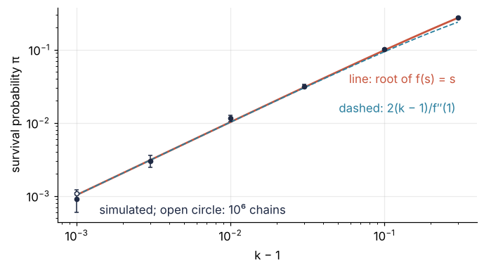
Survival probability against k − 1 from 10⁻³ to 0.3, log-log. The root of f(s) = s, the linear law 2(k − 1)/f″(1), and simulated chains with error bars agree; the law falls 13 % low at k = 1.3.

Every simulated value lies within two standard errors of the root: 9 lasting chains of 10,000 at k = 1.001 against 10.3 expected, 115 at 1.01 against 103, 1,005 at 1.1 against 984. At k = 1.001 the 10,000 chains are a ±30 % check and prove little. The 10⁶ chains give (1.073 ± 0.033) × 10⁻³ against 1.030 × 10⁻³, 1.3 standard errors high, a ±3 % check (The standard error of the mean explains the ±). The cap of 10,000 neutrons does not bias the count: a chain that reaches it still dies with probability q¹⁰⁰⁰⁰ = 3.336 × 10⁻⁵ at k = 1.001, a bias of 0.003 % against the ±3 % of the largest run.

Where it shows up

Reactor startup and pulsed reactors. A startup source keeps neutrons coming, and a source-range counter, the neutron detector that watches a reactor while it is far below power, sees its count rate grow with the subcritical multiplication 1/(1 − k) as k approaches 1. In a pulsed reactor brought above critical quickly, the delay between reaching the target k and the start of the pulse is random, with the rate Sπ of the waiting-time result.
Population genetics. A new beneficial mutation whose carrier leaves a Poisson-distributed number of copies with mean 1.01 survives with probability about 2 %, Haldane's result of 1927; it is the k − 1 law with f″(1) ≈ 1. A neutral copy, as in Genetic drift, wins only with 1/2N in a population of N diploid individuals.
Epidemics. R₀, the mean number of people one case infects, is the k of an outbreak, and the chance that one introduced case starts a lasting outbreak is π. Lloyd-Smith and colleagues (2005) fitted a negative-binomial number of secondary cases, a Poisson-distributed number whose mean itself varies from case to case, and found that a larger spread at the same R₀ makes most introductions fizzle, the spread table above in another field.
Cell lineages and colonies. A cell that divides at rate b and dies at rate d leaves a lineage that dies out with probability d/b when b > d, the same fixed point in continuous time. The Gillespie algorithm tutorial simulates such birth and death processes event by event.
Polymer gelation. In Flory-Stockmayer theory a growing molecule is a branching tree of bonds, and the gel point is where the mean number of further branches per branch reaches 1. The gel fraction plays the role of π: it comes from a fixed-point equation of the same form and grows linearly past the gel point.

In every case one founder's fate turns first on its chance of having no offspring, which the mean alone never shows.

The question

The idea: a chain dies only if every branch dies

Just above critical: why the chance grows as k − 1

Formalization

See it in code

Where it shows up

Further reading