Monte Carlo failure probability with an error bar: does the shaft fit?

The problem

You know how each input scatters and want the probability that a condition fails, with an error bar on that probability. Monte Carlo sampling gives both: draw many parts from a seeded generator, test the condition on each, and count the failures. The example is a shaft made at 20.00 mm going into a bore made at 20.05 mm, both with a standard deviation of 0.02 mm, and the assembly needs at least 0.01 mm of clearance. Swap in your own distributions and condition; the rest of the code stays.

The code

Copy

import numpy as np
import matplotlib.pyplot as plt
from scipy.stats import norm

# ---- inputs: replace with your own distributions
rng = np.random.default_rng(10)
N = 10_000
shaft = rng.normal(20.00, 0.02, N)                          # mm
bore = rng.normal(20.05, 0.02, N)                           # mm

# ---- condition: replace with your own; any boolean array works
fails = bore - shaft < 0.01                                 # too little clearance

# ---- estimate and standard error
p = fails.mean()
se = np.sqrt(p * (1 - p) / N)

# ---- exact check: only for this linear case, delete for your own
sd_clearance = np.sqrt(0.02**2 + 0.02**2)                   # variances of independent parts add
p_exact = norm.cdf(0.01, loc=0.05, scale=sd_clearance)

# ---- samples for a target relative error
r = 0.01                                                    # r = se / p
N_needed = (1 - p) / (p * r**2) if p > 0 else np.inf

# ---- report and plot
print(f"failures: {fails.sum():,} of {N:,}")
if p == 0:                                                  # se is zero too: report a bound, see Pitfalls
    print(f"p < {3 / N:.1e} at 95 % (rule of three)")
else:
    print(f"p = {100 * p:.2f} % ± {100 * se:.2f} %")
    print(f"exact {100 * p_exact:.2f} % ({abs(p - p_exact) / se:.2f} standard errors away)")
    print(f"for {100 * r:.0f} % relative error: about {N_needed:,.0f} samples")

n = np.arange(1, N + 1)
running = np.cumsum(fails) / n
se_running = np.sqrt(running * (1 - running) / n)          # the error bar a run stopped at n reports
keep = n >= 100                                             # the formula is unreliable for fewer samples

fig, ax = plt.subplots(figsize=(7, 3.6), dpi=110)
for k, alpha in [(2, 0.15), (1, 0.30)]:
    ax.fill_between(n[keep], 100 * (running - k * se_running)[keep],
                    100 * (running + k * se_running)[keep], color="#c8553d", alpha=alpha, lw=0)
ax.plot(n[keep], 100 * running[keep], color="#c8553d", lw=1.8)
ax.axhline(100 * p_exact, color="#1f2a44", lw=1.0)
ax.text(1.01, 100 * p_exact, f"exact\n{100 * p_exact:.2f} %", color="#1f2a44", va="center",
        transform=ax.get_yaxis_transform())                # right of the axes, clear of the bands
ax.text(N, 100 * p + 1.2, f"{100 * p:.2f} % ± {100 * se:.2f} %", color="#c8553d", ha="right")
ax.set(xscale="log", xlim=(100, N), xlabel="N / samples", ylabel="failure probability / %")
ax.spines[["top", "right"]].set_visible(False)
plt.show()

failures: 764 of 10,000
p = 7.64 % ± 0.27 %
exact 7.86 % (0.85 standard errors away)
for 1 % relative error: about 120,890 samples

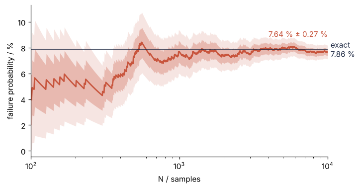
The exact value is there only to check the code. The clearance bore − shaft is itself normal, with mean 0.05 mm and standard deviation √(0.02² + 0.02²) = 0.028 mm, because variances of independent values add, for a difference as for a sum. norm.cdf is the area of that distribution below 0.01 mm, as in scipy.stats from the ground up. The estimate of 7.64 % misses the exact 7.86 % by 0.85 standard errors, a typical miss, since the standard error is the size of miss to expect from a run of this length. The last printed line comes back below.

The two shades in the figure, ±1 and ±2 standard errors, are not drawn around the exact value. At each n they come from that n's own running estimate, so they are the error bars the run would have reported had you stopped there. They narrow as 1/√N, and the estimate wanders inside them.

The knobs

N sets the error bar. A part that fails with probability p is a value that is 1 with probability p and 0 otherwise, whose variance is p(1 − p), so the failure probability is a mean of zeros and ones and its standard error is √(p(1 − p)/N). Solved for N, a relative error r = se/p needs (1 − p)/(p r²) samples: 120,890 for 1 % here, the last printed line, twelve times what the run drew. Rare failures make this explode. At p = 10⁻⁴ the same 1 % needs 10⁸ samples, and that is where importance sampling, which draws more often where the failures are, takes over. Why the error falls as 1/√N however many inputs you have is the subject of Monte Carlo integration. The distributions and the condition are your model: any rng distribution for the inputs, any boolean array for the condition, including ones with no closed form, such as a press fit whose interference depends on the temperature of both parts. For such a condition the exact-check line goes, and the error bar is the only check you have.

The number is a probability under the distributions you assumed, not the reject rate of the plant. If the real diameters have heavier tails than a normal distribution, or the drill for the bores drifts over a shift, the 7.6 % inherits that error, and no N fixes it. The ± is the statistical error of the sampling and nothing else. It says how well 10,000 draws pin down the failure probability of your model, not how well the model describes the parts on the bench.

Pitfalls

Zero failures is not zero probability. Make the same parts to a standard deviation of 0.007 mm instead of 0.02 mm and the exact failure probability drops to 2.7 × 10⁻⁵. With seed 10 the 10,000 draws contain no failure at all, and the formula gives p = 0 ± 0, a zero error for a zero estimate. The code therefore reports an upper bound when the count is zero, the rule of three: p < 3/N = 3 × 10⁻⁴ at 95 %. It is the p for which zero failures in N draws still happen 5 % of the time, (1 − p)^N = 0.05, which for small p gives p ≈ −ln 0.05 / N = 3.0/N. It holds only for a count of zero; otherwise raise N until a few dozen failures turn up.

Correlated inputs drawn independently. Nothing in the output shows this one. Say shaft and bore come off the same machine and share half their variance: a common offset with a standard deviation of 0.014 mm, drawn once per pair, plus each part's own scatter of 0.014 mm, a correlation of 0.5. The offset moves both parts together and cancels in bore − shaft, so the clearance's standard deviation drops to 0.020 mm and p to 2.3 %, against 7.6 % from independent draws. For a sum the same offset adds: two parts stacked against a length limit fail more often, not less. Draw the shared source once per pair, as in the standard error tutorial, or use rng.multivariate_normal with the correlation, as in Uncertainty propagation by sampling.

More digits than the error bar allows. A report of 7.640 % claims four digits from a run whose standard error of 0.27 percentage points already makes the second one uncertain. Seeds 1 to 10 put the estimate anywhere from 7.40 % to 8.28 %. Write 7.6 % ± 0.3 %.