Critical heat flux in a fuel rod: a boiling crisis with solve_ivp (Python)

The problem: a fuel rod past the critical heat flux

Take one slice of a fuel rod in a pressurized-water reactor: a uranium dioxide pellet 4.1 mm in radius, a helium gap of 0.08 mm, and Zircaloy cladding out to 4.75 mm, in water at 15.5 MPa, which boils at 345 °C, its saturation temperature. At the nominal 20 kW per meter of rod, 670 kW/m² leave the cladding surface. The first is the linear heat rate \(q'\), per meter of rod, the second the surface heat flux \(q''\), per square meter of surface; the heat made per cubic meter of fuel is the volumetric heating \(q'''\).

The heat leaves by nucleate boiling, bubbles that form on the wall and carry it off while the wall stays 3.1 K above saturation. That works up to the critical heat flux, here 1.5 MW/m², also called departure from nucleate boiling (DNB). Critical heat flux over actual flux is the DNBR, 2.24 at nominal power.

Now push the power up. In this tutorial's stylized history it ramps until the reactor trips, the automatic shutdown, at three times nominal. The surface flux lags behind, since the pellet stores heat first, but reaches the critical heat flux before the trip. A vapor film then covers the cladding, film boiling, the heat transfer coefficient drops from 321 to 2 kW/(m² K), and the pellet keeps pushing out its stored heat. The rod follows the heat equation in cylindrical coordinates,

\[ \rho c_p \frac{\partial T}{\partial t} = \frac{1}{r}\frac{\partial}{\partial r}\left(r\,k\,\frac{\partial T}{\partial r}\right) + q''' , \]

with density \(\rho\), specific heat \(c_p\), and conductivity \(k\), the last two functions of temperature, and the boiling curve, flux against wall temperature, as the condition at the outer surface.

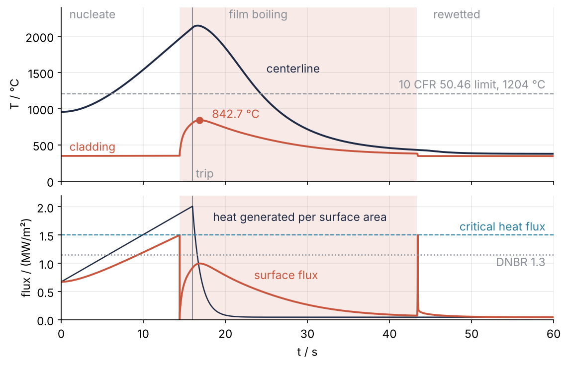
Top: pellet centerline and outer cladding temperature in °C against time in s; only the film boiling phase is shaded. Bottom: surface heat flux in MW/m² against the critical heat flux. The cladding jumps when the flux reaches 1.5 MW/m² at 14.4 s and peaks at 843 °C after the trip at 16 s.

This is where we end up: the cladding jumps when its surface flux reaches the critical heat flux at 14.4 s and peaks at 842.7 °C after the trip; Step 6 explains the 1204 °C and DNBR 1.3 lines. The last of six steps draws this figure.

Setup

Temperatures are in kelvin inside the code and in degrees Celsius in every print. The power history is stylized: a ramp at 2.5 kW/m per second, a trip at 60 kW/m, and a fall with a 1 s time constant to decay heat, the heat the radioactive fission products keep releasing after the chain reaction stops, 6.5 % of nominal and held constant here.

import numpy as np
import matplotlib.pyplot as plt
from scipy.integrate import solve_ivp

K = 273.15                       # 0 °C in kelvin

# one axial slice of a pressurized-water-reactor fuel rod
r_p = 4.1e-3                     # pellet radius, m
r_ci, r_co = 4.18e-3, 4.75e-3    # cladding inside and outside radius, m; the helium gap is 0.08 mm
p = 15.5                         # coolant pressure, MPa
T_sat = 345.0 + K                # saturation temperature of water at 15.5 MPa, K
q_chf = 1.5e6                    # critical heat flux, W/m²
h_gap = 6e3                      # gap conductance, W/(m² K)
h_film = 2e3                     # film boiling heat transfer coefficient, W/(m² K)
T_min = 380.0 + K                # minimum film boiling temperature, K
rho_f = 0.95 * 10960             # UO2 at 95 % of theoretical density, kg/m³
rho_c, cp_c = 6550.0, 330.0      # Zircaloy-4: density kg/m³, specific heat J/(kg K)

# the stylized power history
q0 = 20e3                        # nominal linear heat rate, W/m
ramp, q_trip = 2.5e3, 60e3       # rise in W/m per s, and the level at which the reactor trips, W/m
t_trip = (q_trip - q0) / ramp

def power(t):
    """Linear heat rate in W/m: ramp, trip, and a fall with a 1 s time constant to 6.5 % decay heat."""
    after = 0.065 * q0 + (q_trip - 0.065 * q0) * np.exp(-(t - t_trip) / 1.0)
    return np.where(t < t_trip, q0 + ramp * t, after)

plt.rcParams.update({                      # the look of every figure below
    "figure.figsize": (7, 3.6), "figure.dpi": 110,
    "axes.spines.top": False, "axes.spines.right": False,
    "axes.grid": True, "grid.alpha": 0.25,
    "font.size": 11, "lines.linewidth": 1.8,
})
INK, ACCENT, SECOND, MUTED = "#1f2a44", "#c8553d", "#2a7f9e", "#8a8f98"

q_nominal = q0 / (2 * np.pi * r_co)
print(f"trip at t = {t_trip:.1f} s; nominal surface flux {q_nominal / 1e3:.0f} kW/m², DNBR {q_chf / q_nominal:.2f}")

trip at t = 16.0 s; nominal surface flux 670 kW/m², DNBR 2.24

Step 1: Compute the steady state from the surface inward

At constant power every watt made in the pellet crosses the pellet, the gap, the cladding, and the boiling wall, and each layer costs a temperature drop, added up from the water inward. At the wall, Thom's correlation for nucleate boiling, a mild extrapolation from data up to about 14 MPa, gives \(T_w - T_\mathrm{sat} = 22.65\,\sqrt{q''}\,e^{-p/8.7}\), with \(q''\) in MW/m² and the pressure \(p\) in MPa. The gap is a contact conductance \(h_\mathrm{gap}\), a drop of \(q'/(2\pi r_p h_\mathrm{gap})\).

In the cladding and the pellet the heat crossing radius \(r\) is known too: all of \(q'\) in the cladding, the part made inside \(r\) in the pellet. Fourier's law becomes a first-order ODE in \(r\),

\[ \frac{dT}{dr} = -\frac{q'}{2\pi r\,k(T)}\ \ \text{(cladding)}, \qquad \frac{dT}{dr} = -\frac{q''' r}{2\,k(T)}\ \ \text{(pellet)}, \]

which solve_ivp integrates with \(r\) in place of \(t\). The span (r_co, r_ci) runs inward, and the solver steps backward. The pellet form has no \(1/r\), so it runs to \(r = 0\).

def k_fuel(T):
    """UO2 at 95 % density, Fink (2000), W/(m K)."""
    tau = T / 1000
    return 100 / (7.5408 + 17.692 * tau + 3.6142 * tau**2) + 6400 / tau**2.5 * np.exp(-16.35 / tau)

def k_clad(T):
    """Zircaloy-4, MATPRO, W/(m K)."""
    return 7.51 + 2.09e-2 * T - 1.45e-5 * T**2 + 7.67e-9 * T**3

C_thom = np.exp(2 * p / 8.7) / 22.65**2 * 1e6       # Thom solved for the flux: q'' = C (Tw - T_sat)², W/(m² K²)

def nucleate(Tw):
    dT = Tw - T_sat
    return C_thom * dT * np.abs(dT)                   # keeps its sign: a wall below saturation takes heat in

T_co = T_sat + np.sqrt(q_nominal / C_thom)
clad = solve_ivp(lambda r, T: -q0 / (2 * np.pi * r * k_clad(T)), (r_co, r_ci), [T_co], rtol=1e-10, atol=1e-10)
T_ci = clad.y[0, -1]
T_ps = T_ci + q0 / (2 * np.pi * r_p * h_gap)
q_vol = q0 / (np.pi * r_p**2)                       # volumetric heating, W/m³
pellet = solve_ivp(lambda r, T: -q_vol * r / (2 * k_fuel(T)), (r_p, 0), [T_ps], rtol=1e-10, atol=1e-10)
T_c = pellet.y[0, -1]

steady = {"cladding outside": T_co, "cladding inside": T_ci, "pellet surface": T_ps, "pellet center": T_c}
for (name, T), drop in zip(steady.items(), np.diff([T_sat, *steady.values()])):
    print(f"{name:17s} {T - K:6.1f} °C   {drop:6.1f} K above the layer outside it")
print(f"UO2 conducts {k_fuel(T_ps):.2f} W/(m K) at the pellet surface, {k_fuel(T_c):.2f} W/(m K) at the center")

cladding outside   348.1 °C      3.1 K above the layer outside it
cladding inside    372.2 °C     24.1 K above the layer outside it
pellet surface     501.6 °C    129.4 K above the layer outside it
pellet center      956.5 °C    454.9 K above the layer outside it
UO2 conducts 4.27 W/(m K) at the pellet surface, 2.88 W/(m K) at the center

The boiling wall costs 3.1 K, the cladding 24.1 K, the gap 129.4 K, and the pellet 454.9 K. The 0.08 mm of helium costs five times as much as the 0.57 mm of metal, and the pellet most, because UO2 conducts poorly and worse when hot, 2.88 W/(m K) at its center. These four temperatures test every later step.

Step 2: Lay a radial grid over pellet and cladding

The grid follows the planetary tutorial: nodes, each owning the material halfway to its neighbors. Here 25 nodes run from \(r = 0\) to the pellet surface and six from the inside of the cladding to its outside, with a node on each surface, because the gap and the boiling curve need surface temperatures. In a cylinder the layers are rings: per meter of rod a node owns the volume \(\pi(r_\mathrm{out}^2 - r_\mathrm{in}^2)\) between its faces and exchanges heat through faces of area \(2\pi r_f\).

The center node owns a disk, and its inner face at \(r = 0\) has zero area, so no heat crosses it and nothing is ever divided by \(r\). That is how a finite-volume grid deals with the \(1/r\) of the heat equation; the finite volumes tutorial explains the bookkeeping. The gap gets no node; it is a conductance between the last pellet node and the first cladding node, \(Q_\mathrm{gap} = 2\pi r_p h_\mathrm{gap}(T_{ps} - T_{ci})\) in W per meter of rod, with \(T_{ps}\) and \(T_{ci}\) the pellet surface and the cladding inside.

n_f, n_c = 25, 6
r = np.r_[np.linspace(0, r_p, n_f), np.linspace(r_ci, r_co, n_c)]   # node radii, m
face_f = (r[:n_f - 1] + r[1:n_f]) / 2                              # faces between pellet nodes
face_c = (r[n_f:-1] + r[n_f + 1:]) / 2                             # faces between cladding nodes
inner = np.r_[0.0, face_f, r_ci, face_c]                           # inner face of each node
outer = np.r_[face_f, r_p, face_c, r_co]                           # outer face of each node
V = np.pi * (outer**2 - inner**2)                                  # volume per meter of rod, m²

print(f"{r.size} nodes; spacing {1e3 * (r[1] - r[0]):.3f} mm in the pellet, {1e3 * (r[-1] - r[-2]):.3f} mm in the cladding")
print(f"pellet volumes / (π r_p²)          = {V[:n_f].sum() / (np.pi * r_p**2):.12f}")
print(f"cladding volumes / π(r_co² - r_ci²) = {V[n_f:].sum() / (np.pi * (r_co**2 - r_ci**2)):.12f}")

31 nodes; spacing 0.171 mm in the pellet, 0.114 mm in the cladding
pellet volumes / (π r_p²)          = 1.000000000000
cladding volumes / π(r_co² - r_ci²) = 1.000000000000

The rings tile pellet and cladding without a hole or an overlap, to twelve digits. The nodes on the three surfaces own half cells, as in the planetary grid, and so does the center.

Step 3: Write one ODE per node with k(T) at the faces

Per meter of rod, node \(i\) changes its heat content by what flows in, minus what flows out, plus what it makes:

\[ \rho c_p(T_i)\,V_i\,\frac{dT_i}{dt} = Q_{\mathrm{in},i} - Q_{\mathrm{out},i} + q'''\,V_i , \]

the balance of the planetary tutorial with rings in place of layers. Each face carries Fourier's law, \(Q = -2\pi r_f\,k\,\Delta T/\Delta r\), with \(k\) at the face temperature, the mean of the two neighbors. The specific heat of UO2 is Fink's, that of Zircaloy constant, and the source \(q'(t)/(\pi r_p^2)\) heats the pellet only. rhs receives the surface flux and the power history as functions, through args=(surface, power): Step 5 swaps the surface function, and here the power is a constant.

def cp_fuel(T):
    """UO2, Fink (2000), J/(kg K)."""
    C1, theta, C2, C3, Ea = 81.613, 548.68, 2.285e-3, 2.360e7, 18531.7
    e = np.exp(theta / T)
    per_mole = C1 * theta**2 * e / (T**2 * (e - 1) ** 2) + 2 * C2 * T + C3 * Ea * np.exp(-Ea / T) / T**2
    return per_mole / 0.27003                        # J/(mol K) to J/(kg K)

def rhs(t, T, surface, power):
    T_f, T_cl = T[:n_f], T[n_f:]
    # heat through each face in W per meter of rod, with k at the face temperature
    Q_f = -2 * np.pi * face_f * k_fuel((T_f[:-1] + T_f[1:]) / 2) * np.diff(T_f) / np.diff(r[:n_f])
    Q_c = -2 * np.pi * face_c * k_clad((T_cl[:-1] + T_cl[1:]) / 2) * np.diff(T_cl) / np.diff(r[n_f:])
    Q_gap = 2 * np.pi * r_p * h_gap * (T_f[-1] - T_cl[0])
    Q_surface = 2 * np.pi * r_co * surface(T[-1])
    Q = np.r_[0.0, Q_f, Q_gap, Q_c, Q_surface]       # Q[i] enters node i, Q[i + 1] leaves it
    source = np.r_[np.full(n_f, power(t) / (np.pi * r_p**2)), np.zeros(n_c)] * V
    capacity = np.r_[rho_f * cp_fuel(T_f), np.full(n_c, rho_c * cp_c)] * V
    return (Q[:-1] - Q[1:] + source) / capacity

Started from a flat 345 °C and run for 100 s at nominal power, the rod must settle into the steady state of Step 1. The same cell estimates how fast the outermost node responds: its heat capacity \(\rho c_p V\) over the conductance that drains it, to its inner neighbor and to the water. The water's share is the slope \(dq''/dT_w\) of the boiling curve times the surface area.

run = solve_ivp(rhs, (0, 100), np.full(r.size, T_sat), method="BDF",
                args=(nucleate, lambda t: q0), rtol=1e-8, atol=1e-6)
T0 = run.y[:, -1]                                    # the nominal state, the start of the transient
for (name, T), i in zip(steady.items(), [-1, n_f, n_f - 1, 0]):
    print(f"{name:17s} {T0[i] - K:6.1f} °C   ({T0[i] - T:+.3f} K against Step 1)")

conductance = (2 * np.pi * face_c[-1] * k_clad(T0[-2:].mean()) / (r[-1] - r[-2])    # to the inner neighbor
               + 2 * np.pi * r_co * 2 * C_thom * (T0[-1] - T_sat))                 # to the water, dq''/dTw
tau_out = rho_c * cp_c * V[-1] / conductance
print(f"outer node settles in {1e3 * tau_out:.2f} ms, {100 / tau_out:,.0f} times shorter than the 100 s run")

cladding outside   348.1 °C   (+0.000 K against Step 1)
cladding inside    372.2 °C   (-0.001 K against Step 1)
pellet surface     501.6 °C   (-0.001 K against Step 1)
pellet center      956.5 °C   (+0.018 K against Step 1)
outer node settles in 0.21 ms, 469,200 times shorter than the 100 s run

The grid reproduces Step 1 to 0.018 K at the center and better elsewhere. The outer node settles in 0.21 ms, a time scale about 470,000 times shorter than the 100 s run: a stiff system, as in the stiffness tutorial, and the reason for BDF.

Step 4: Put the boiling curve on the outer surface

The boiling curve has two branches. The wet one follows Thom up to the critical heat flux, then a stylized transition line, straight on linear axes, down to the minimum film boiling temperature \(T_\mathrm{min} = 380\) °C, also called the Leidenfrost temperature: the coldest wall that can hold a vapor film, the reason a drop skates on a hot pan. There the line ends at \(q_\mathrm{min} = h_\mathrm{film}(T_\mathrm{min} - T_\mathrm{sat})\). The film branch is \(h_\mathrm{film}(T_w - T_\mathrm{sat})\) with 2 kW/(m² K).

A heated wall never walks the transition line. At the critical heat flux it drops onto the film branch and stays there until it cools below \(T_\mathrm{min}\); only then does it rewet, water touching the wall again, and travel up the transition line as it cools. The two arrows in the figure trace this loop. Between the crisis temperature and 380 °C both branches exist, and which one holds depends on where the wall came from. That is hysteresis, and the reason the regime must live outside rhs.

T_chf = T_sat + np.sqrt(q_chf / C_thom)             # where Thom reaches the critical heat flux
q_min = h_film * (T_min - T_sat)

def wet(Tw):
    return np.where(Tw < T_chf, nucleate(Tw), np.interp(Tw, [T_chf, T_min], [q_chf, q_min]))

def film(Tw):
    return h_film * (Tw - T_sat)

print(f"crisis at {T_chf - K:.1f} °C, q_min = {q_min / 1e3:.0f} kW/m²")
print(f"at the crisis: wet {q_chf / (T_chf - T_sat) / 1e3:.0f} kW/(m² K), film {h_film / 1e3:.0f} kW/(m² K); "
      f"film flux {film(T_chf) / 1e3:.1f} kW/m², {q_chf / film(T_chf):.0f} times less")

dT = np.geomspace(0.5, 600, 500)                    # wall superheat, K
Tw = T_sat + dT
fig, ax = plt.subplots()
ax.loglog(dT[Tw <= T_min], wet(Tw[Tw <= T_min]), color=INK)
ax.loglog(dT[Tw >= T_chf], film(Tw[Tw >= T_chf]), color=ACCENT)
ax.axhline(q_chf, color=SECOND, ls="--", lw=1)
ax.axvline(T_min - T_sat, color=MUTED, ls="--", lw=1)
arrow = dict(arrowstyle="->", color=MUTED, lw=1.2)
x_chf = T_chf - T_sat
ax.annotate("", xy=(x_chf, 1.3 * film(T_chf)), xytext=(x_chf, 0.8 * q_chf), arrowprops=arrow)        # heating: the crisis
ax.text(0.9 * x_chf, 1.0e5, "heating", color=MUTED, ha="right")
x_up = np.geomspace(31, 7, 40)                                                                     # cooling: up the transition line
ax.plot(x_up, 0.55 * wet(T_sat + x_up), color=MUTED, lw=1.2)
ax.annotate("", xy=(x_up[-1], 0.55 * wet(T_sat + x_up[-1])), xytext=(x_up[-2], 0.55 * wet(T_sat + x_up[-2])), arrowprops=arrow)
ax.text(10, 2.2e5, "cooling", color=MUTED)
ax.text(0.6, 2.5e5, "nucleate\n(Thom)", color=INK)
ax.text(38, 4e5, "transition", color=INK)
ax.text(120, 1.0e5, "film boiling", color=ACCENT)
ax.text(70, 1.8e6, "critical heat flux", color=SECOND)
ax.text(1.05 * (T_min - T_sat), 5e3, "$T_\\mathrm{min}$", color=MUTED)
ax.set(xlabel="wall superheat $T_w - T_\\mathrm{sat}$ / K", ylabel="surface heat flux / (W/m²)",
       xlim=(0.5, 600), ylim=(3e3, 1e7))
plt.show()

crisis at 349.7 °C, q_min = 70 kW/m²
at the crisis: wet 321 kW/(m² K), film 2 kW/(m² K); film flux 9.3 kW/m², 161 times less

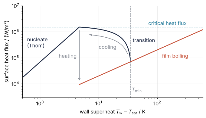
Boiling curve on log-log axes: surface heat flux in W/m² against wall superheat in K. The wet branch rises to the critical heat flux of 1.5 MW/m², then falls along the transition line to 380 °C; arrows show a heated wall jumping down to the film branch at the critical heat flux, and a cooling wall leaving it at 380 °C and climbing the transition line.

Thom reaches the critical heat flux at 349.7 °C, 4.7 K above saturation, with an effective coefficient of 321 kW/(m² K) against the film's 2. At the moment of the crisis the same wall at the same temperature passes on 9.3 kW/m² instead of 1.5 MW/m², 161 times less.

Step 5: Switch the regime with terminal events

Two events mark the switches. The crisis is the zero of nucleate(T[-1]) - q_chf, crossed upward. The rewet is the zero of T[-1] - T_min, crossed downward, and the direction matters: right after the crisis the wall is at 349.7 °C and climbs through \(T_\mathrm{min}\) before it can come back down. Both are terminal and accept the args of rhs, as every event function must.

The loop runs solve_ivp from the current time and state to 60 s with the surface function and event of the current regime. sol.status says why a run ended: 0 means it reached the end, the only case the solve_ivp tutorial met, and 1 means a terminal event stopped it. On 1 the loop flips the regime and restarts from sol.t[-1] and sol.y[:, -1]. A restart sits on the zero of the event that stopped it, and an event that starts at zero can fire again at once. Here it cannot: the new regime watches the other event, far from zero.

def crisis(t, T, surface, power):
    return nucleate(T[-1]) - q_chf
crisis.terminal, crisis.direction = True, 1

def rewet(t, T, surface, power):
    return T[-1] - T_min
rewet.terminal, rewet.direction = True, -1          # down through T_min, not up through it after the crisis

regimes = {"nucleate": (wet, crisis, "film"), "film": (film, rewet, "nucleate")}
t, T, regime = 0.0, T0, "nucleate"
segments, switches = [], []
while True:
    surface, event, after = regimes[regime]
    sol = solve_ivp(rhs, (t, 60.0), T, method="BDF", args=(surface, power), events=event, rtol=1e-6, atol=1e-6)
    segments.append((regime, sol))
    if sol.status != 1:                              # 0: the end of the run, no event
        break
    t, T = sol.t[-1], sol.y[:, -1]
    switches.append(t)
    print(f"{regime:>8s} to {after:8s} at t = {t:5.2f} s: cladding {T[-1] - K:5.1f} °C, power {power(t) / 1e3:4.1f} kW/m")
    regime = after

steps = sum(s.t.size - 1 for _, s in segments)
print(f"{len(segments)} segments, {steps} steps, nfev {sum(s.nfev for _, s in segments)}")

nucleate to film     at t = 14.43 s: cladding 349.7 °C, power 56.1 kW/m
    film to nucleate at t = 43.35 s: cladding 380.0 °C, power  1.3 kW/m
3 segments, 395 steps, nfev 966

The crisis comes at 14.43 s, 1.6 s before the trip, with the power rising at 56.1 kW/m. The wall rewets at 43.35 s, at 1.3 kW/m of decay heat. The minute takes 395 steps and 966 calls of rhs, not counting those that build the Jacobian.

Step 6: Find the peak cladding temperature and draw the transient

Join the segments; the surface flux comes from each segment's branch. Two limits go into the figure. The design limit keeps the DNBR above about 1.3, so that the crisis is never approached, and the time it fell below is interpolated on the first segment, where the flux only rises. The 1204 °C line is the peak cladding temperature criterion of 10 CFR 50.46, written for a loss-of-coolant accident and only a yardstick here.

t_all = np.concatenate([s.t for _, s in segments])
T_all = np.hstack([s.y for _, s in segments])
q_all = np.concatenate([regimes[reg][0](s.y[-1]) for reg, s in segments])   # surface flux, W/m²
t_crisis, t_rewet = switches

i, j = T_all[-1].argmax(), T_all[0].argmax()
first = segments[0][1]
t_13 = np.interp(q_chf / 1.3, wet(first.y[-1]), first.t)
print(f"peak cladding   {T_all[-1, i] - K:6.1f} °C at {t_all[i]:5.2f} s, {t_all[i] - t_trip:.2f} s after the trip")
print(f"peak centerline {T_all[0, j] - K:6.0f} °C at {t_all[j]:5.2f} s")
print(f"film boiling for {t_rewet - t_crisis:.1f} s; DNBR below 1.3 from {t_13:.2f} s at {power(t_13) / 1e3:.1f} kW/m")

fig, (ax1, ax2) = plt.subplots(2, 1, sharex=True, figsize=(7.5, 4.8), height_ratios=[2.8, 2], layout="constrained")
for ax in (ax1, ax2):
    ax.axvspan(t_crisis, t_rewet, color=ACCENT, alpha=0.12, lw=0)
    ax.axvline(t_trip, color=MUTED, lw=1)
ax1.plot(t_all, T_all[0] - K, color=INK)
ax1.plot(t_all, T_all[-1] - K, color=ACCENT)
ax1.plot(t_all[i], T_all[-1, i] - K, "o", color=ACCENT, ms=6)
ax1.text(t_all[i] + 1.5, T_all[-1, i] - K + 30, f"{T_all[-1, i] - K:.1f} °C", color=ACCENT)
ax1.axhline(1204, color=MUTED, ls="--", lw=1)
ax1.text(59, 1280, "10 CFR 50.46 limit, 1204 °C", color=MUTED, ha="right")
ax1.text(25, 1500, "centerline", color=INK)
ax1.text(1, 420, "cladding", color=ACCENT)
for x, name in [(1, "nucleate"), (t_crisis + 6, "film boiling"), (t_rewet + 2, "rewetted")]:
    ax1.text(x, 2250, name, color=MUTED)
ax1.text(t_trip + 0.4, 50, "trip", color=MUTED)
ax1.set(ylabel="T / °C", ylim=(0, 2400))

tt = np.linspace(0, 60, 1201)
ax2.plot(tt, power(tt) / (2 * np.pi * r_co) / 1e6, color=INK, lw=1.2)
ax2.plot(t_all, q_all / 1e6, color=ACCENT)
ax2.axhline(q_chf / 1e6, color=SECOND, ls="--", lw=1)
ax2.axhline(q_chf / 1.3 / 1e6, color=MUTED, ls=":", lw=1.2)
ax2.text(59, 1.58, "critical heat flux", color=SECOND, ha="right")
ax2.text(59, 0.95, "DNBR 1.3", color=MUTED, ha="right")
ax2.text(18.5, 1.75, "heat generated per surface area", color=INK)
ax2.text(23.5, 0.72, "surface flux", color=ACCENT)
ax2.set(xlabel="t / s", ylabel="flux / (MW/m²)", xlim=(0, 60), ylim=(0, 2.2))
plt.show()

peak cladding    842.7 °C at 16.87 s, 0.87 s after the trip
peak centerline   2148 °C at 16.63 s
film boiling for 28.9 s; DNBR below 1.3 from 9.43 s at 43.6 kW/m

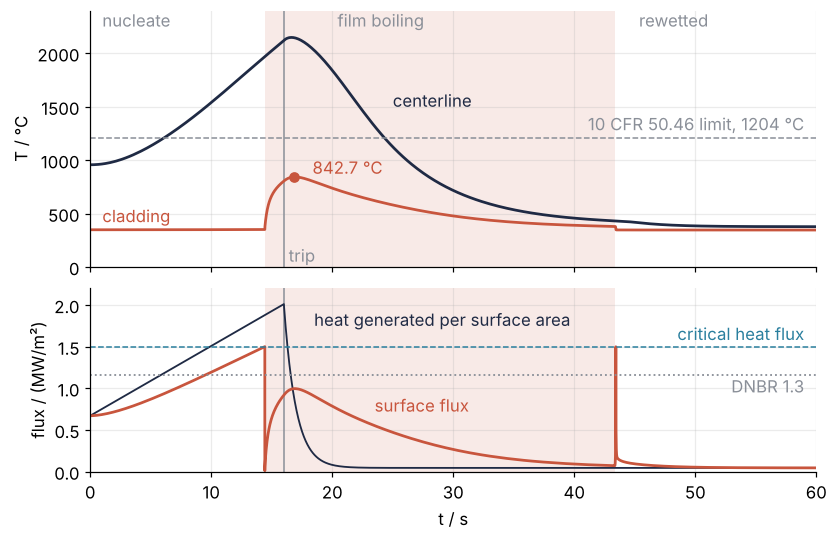
Top: centerline and cladding temperature in °C against time in s; only the film boiling phase is shaded. Bottom: surface heat flux in MW/m². The flux passes the DNBR 1.3 line at 9.4 s, the cladding jumps at 1.5 MW/m² at 14.4 s, peaks at 843 °C after the trip, and falls back after the rewet at 43 s.

The cladding peaks at 842.7 °C at 16.87 s, 0.87 s after the trip: the power is falling, but the pellet, 2148 °C at its center, keeps emptying its heat into a surface that takes little away. The spike of the surface flux back to 1.5 MW/m² at 43 s is the quench, not a second crisis. The rewetted wall cools from 380 °C up the transition line, and the cladding's stored heat leaves at nearly the critical heat flux for a moment.

This history crossed DNBR 1.3 at 9.43 s, 6.6 s before the trip, and reached the crisis itself, DNBR 1, at 14.43 s; the peak stays 361 K under 1204 °C. A real plant trips at about 109 % power, long before either DNBR line.

This is a teaching model with a stylized history and literature properties, not a licensing calculation; system codes such as RELAP5 and TRACE and fuel performance codes such as FRAPTRAN and BISON do that job. The constant \(c_p\) of Zircaloy ignores the α-β phase change that starts near 820 °C, which the peak just touches, and the reaction of Zircaloy with steam, left out, is negligible below about 1000 °C. Four times the nodes move the peak by 0.5 K.

Pitfalls

An if inside rhs instead of an event. Use nucleate(Tw) if Tw < T_chf else film(Tw) as the surface function and integrate the minute in one call. Around 14.43 s BDF cuts its steps down to 2.3 µs, 15 of them under 0.1 ms, to get past the jump in the right-hand side. The peak agrees with Step 6 to 0.04 K, which hides the real damage: the cladding never rewets. A function of the present temperature cannot remember which branch it is on, so this one leaves film boiling only below 349.7 °C, and the decay heat holds the wall in film boiling at 367.6 °C at 60 s. Keep the regime in the loop and let events find the switches.

Forgetting the hysteresis. Two versions of the same mistake. Rewet when the heat generated per surface area falls below the critical heat flux, and the switch comes at 16.30 s with the cladding at 826.8 °C, 447 K above \(T_\mathrm{min}\), where no correlation for a wet wall applies. Leave out direction = -1, and the rewet fires 12 ms after the crisis, on the way up through 380 °C. Both have one cause: they let the wall leave film boiling somewhere other than on its way down through \(T_\mathrm{min}\). The fix is the event of Step 5, the wall temperature with its direction.

Dividing by r at the center. Write the finite-difference form of \(\frac{1}{r}\partial_r(rk\,\partial_r T)\) with np.gradient on the pellet nodes and evaluate it at the center node: NumPy warns "divide by zero encountered in divide", the center's rate is -inf, and BDF gives up before its first step with "array must not contain infs or NaNs". The \(1/r\) is singular at \(r = 0\) although the temperature there is smooth. The finite-volume center node of Step 2, whose inner face has zero area, never divides by \(r\); a finite-difference code uses the limit \(2k\,\partial_r^2 T\) at \(r = 0\) instead.

Variations

A worse film coefficient. Set h_film = 1000, and the peak rises to 1063 °C with no rewet within 60 s, because \(q_\mathrm{min}\) falls to 35 kW/m², below the decay-heat flux of 43.6 kW/m². At 3000 W/(m² K) the peak is 727 °C and the rewet comes at 35.6 s.
Loss of flow. When the pumps slow down, the critical heat flux falls while the power stays put. Make q_chf a function of t in the crisis event and in wet, and keep the power at nominal.
A critical heat flux from a table. Replace the constant q_chf by the 2006 look-up table of Groeneveld and coworkers at 15.5 MPa, your mass flux, and a quality of 0, interpolated with scipy.interpolate.RegularGridInterpolator.
Point kinetics instead of a prescribed history. Let the neutron population set the power, with Doppler feedback from the pellet's mean temperature: hotter fuel absorbs more neutrons without fission and slows the chain reaction. Each group of delayed-neutron precursors, fission products that release a neutron seconds to a minute later, adds one ODE to the same rhs.

Cheat sheet

V = np.pi * (np.r_[faces, r_out]**2 - np.r_[0.0, faces]**2)      # ring volumes per meter; zero area at r = 0, no 1/r
Q = -2 * np.pi * faces * k((T[:-1] + T[1:]) / 2) * np.diff(T) / np.diff(r)   # k at the face temperature
Q_gap = 2 * np.pi * r_p * h_gap * (T_pellet_surface - T_clad_inside)         # the gap is a conductance, not a node
crisis.terminal, crisis.direction = True, 1                      # nucleate(T[-1]) - q_chf, crossed upward
rewet.terminal, rewet.direction = True, -1                       # T[-1] - T_min, crossed downward only
while True:
    surface, event, after = regimes[regime]                      # regimes of Step 5: surface, event, next regime
    sol = solve_ivp(rhs, (t, t_end), T, method="BDF", args=(surface, power), events=event)
    if sol.status != 1: break                                    # 0: reached t_end; 1: a terminal event fired
    t, T, regime = sol.t[-1], sol.y[:, -1], after                # restart from the event on the other branch