The Gillespie algorithm: how noisy is a protein with ten copies per cell? (Python)

The problem: how noisy is a protein that a cell keeps at ten copies?

A bacterium makes a protein at \(k = 1\) molecule per minute, and each molecule is lost, diluted by growth or degraded, at a rate \(\gamma = 0.1\) per minute. The rate equation \(dn/dt = k - \gamma n\) settles at \(n = k/\gamma = 10\), in every cell. With ten molecules, though, every production and every loss is a single random event, and no two cells share a history. The Gillespie algorithm simulates such a history exactly: draw the waiting time to the next reaction from an exponential distribution, pick which reaction it is in proportion to its rate, apply it, repeat.

How far the cells spread is measured by the Fano factor, the variance of the copy number divided by its mean. When molecules are made at a constant rate and lost one at a time, the copy numbers across cells follow a Poisson distribution, and every Poisson distribution has a Fano factor of 1, whatever its mean: a count of 10 has a standard deviation of 3.2, one of 1,000 has 32. Many genes make their protein in bursts instead. At 0.2 bursts per minute of 5 molecules on average, geometrically distributed, the mean is still 10, but theory predicts a Fano factor of 6 and a standard deviation of 7.7.

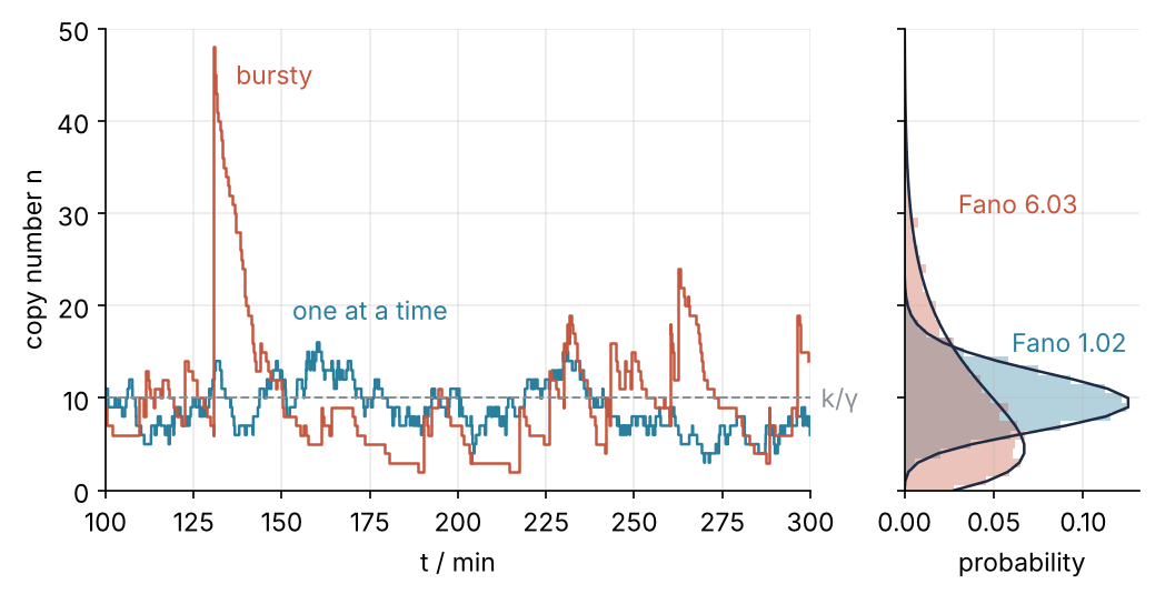
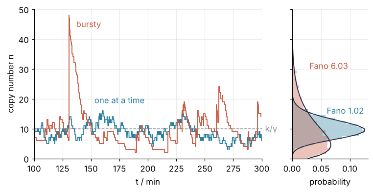
Left: copy number against time in minutes, 100 to 300, for one cell per model; the one-at-a-time cell stays near 10, the bursty cell jumps to 48 and decays back. Right: histograms of 5,000 cells per model on the Poisson and negative binomial curves; Fano factors 1.02 and 6.03.

On the left is one cell of each kind, on the right the copy numbers of 5,000 simulated cells per model with the two theoretical distributions. The measured Fano factors are 1.02 ± 0.02 and 6.03 ± 0.14. Everything in the figure comes from one function of fourteen lines, written in Step 2 and never changed after.

Setup

The rates, one seeded generator for every random draw (the subject of Random numbers with numpy.random), and the style block:

import numpy as np
import matplotlib.pyplot as plt
from scipy import stats

K, GAMMA = 1.0, 0.1         # production per minute, loss per molecule per minute
K_BURST, B_MEAN = 0.2, 5    # bursts per minute, mean burst size
rng = np.random.default_rng(1977)

plt.rcParams.update({
    "figure.figsize": (7, 3.6), "figure.dpi": 110,
    "axes.spines.top": False, "axes.spines.right": False,
    "axes.grid": True, "grid.alpha": 0.25,
    "font.size": 11, "lines.linewidth": 1.8,
})
INK, ACCENT, SECOND, MUTED = "#1f2a44", "#c8553d", "#2a7f9e", "#8a8f98"

print(f"rate-equation steady state k/γ = {K / GAMMA:.0f} molecules")

rate-equation steady state k/γ = 10 molecules

Step 1: Write the reactions as a table of changes and rates

From zero copies the rate equation gives \(n(t) = 10\,(1 - e^{-\gamma t})\), which approaches 10 with a relaxation time \(1/\gamma = 10\) min. You will need that time to know when a simulated cell has forgotten how it started.

For the simulation each reaction needs two things. The first is the change it makes to the copy numbers: one row of the stoichiometry table, with one column per species. The second is its propensity \(a_j\), a rate per minute, not a probability: \(a_j\,dt\) is the chance that reaction \(j\) fires within a short time \(dt\). Production has \(a_1 = k\), loss \(a_2 = \gamma n\).

stoich = np.array([[+1],    # production
                   [-1]])   # loss

def propensities(x):
    return np.array([K, GAMMA * x[0]])

for n in [0, 10, 30]:
    print(f"n = {n:2d}   propensities = {propensities([n])} per min")

n =  0   propensities = [1. 0.] per min
n = 10   propensities = [1. 1.] per min
n = 30   propensities = [1. 3.] per min

The rate equation is the table's changes weighted by the propensities, \(k \cdot (+1) + \gamma n \cdot (-1)\), and at 10 molecules the two cancel. The cell does not stop there. It still gains a molecule about once a minute and loses one about once a minute.

Step 2: Draw the waiting time and the next reaction

Two questions decide what happens next: when, and which reaction. The propensities do not change until some reaction fires, so the chance that some reaction fires in the next short interval \(dt\) stays \(a_0\,dt\), with \(a_0 = \sum_j a_j\) the total propensity, however long the cell has already waited. The one waiting-time distribution with that property is the exponential, with rate \(a_0\), so the mean wait is \(1/a_0\), and rng.exponential(1 / a0) draws it. Which reaction fires is a competition of the rates: reaction \(j\) wins with probability \(a_j/a_0\).

To make that choice, lay the propensities end to end on a line of length \(a_0\), so that reaction \(j\) owns a piece of length \(a_j\). A uniform random point on the line falls into piece \(j\) with probability \(a_j/a_0\). np.cumsum(a) gives the ends of the pieces, and np.searchsorted finds the piece the point fell into. The state then moves by row \(j\) of the table:

def gillespie(x0, stoich, propensities, t_end, rng):
    t, x = 0.0, np.array(x0)
    T, X = [t], [x]
    while True:
        a = propensities(x)
        a0 = a.sum()
        t += rng.exponential(1 / a0)
        if t > t_end:
            break
        j = np.searchsorted(np.cumsum(a), rng.random() * a0, side="right")
        x = x + stoich[j]
        T.append(t)
        X.append(x)
    return np.array(T), np.array(X)

The function propensities is passed in by name like any other argument, so the same loop runs any table of reactions; Step 6 hands it a different one. T holds the event times, and X[i] is the state from T[i] until the next event. Before trusting the loop, check its two draws at \(n = 10\), where \(a_0 = 2\) per minute:

a = propensities([10])
a0 = a.sum()
waits = rng.exponential(1 / a0, size=100_000)
picks = np.searchsorted(np.cumsum(a), rng.random(100_000) * a0, side="right")
print(f"mean wait          {waits.mean():.3f} min   (1/a0 = {1 / a0:.3f})")
print(f"production picked  {np.mean(picks == 0):.3f}       (a1/a0 = {a[0] / a0:.3f})")

mean wait          0.503 min   (1/a0 = 0.500)
production picked  0.498       (a1/a0 = 0.500)

The mean wait is 0.503 min against \(1/a_0 = 0.5\) min, and production wins 49.8 % of the draws against 50 %. Both draws do what the theory says.

Step 3: Simulate one cell from zero copies

One cell, starting from zero copies, for 200 minutes, read now and then with state_at, which returns the state in force at a time \(t\):

def state_at(T, X, t):
    return X[np.searchsorted(T, t, side="right") - 1]   # the last state entered at or before t

T, X = gillespie([0], stoich, propensities, 200, rng)
after = T >= 50
print(f"{len(T) - 1} events in 200 min; after 50 min n ranges from {X[after].min()} to {X[after].max()}")
for t in [5, 30]:
    print(f"t = {t:2d} min   cell {state_at(T, X, t)[0]}   rate equation {K / GAMMA * (1 - np.exp(-GAMMA * t)):.1f}")

349 events in 200 min; after 50 min n ranges from 3 to 19
t =  5 min   cell 8   rate equation 3.9
t = 30 min   cell 6   rate equation 9.5

t_curve = np.linspace(0, 200, 400)
fig, ax = plt.subplots(figsize=(7, 3.2))
ax.step(T, X[:, 0], where="post", color=SECOND, lw=1.2)
ax.plot(t_curve, K / GAMMA * (1 - np.exp(-GAMMA * t_curve)), color=INK)
ax.annotate("rate equation", xy=(10, K / GAMMA * (1 - np.exp(-1))), xytext=(18, 1.5),
            color=INK, arrowprops=dict(arrowstyle="-", color=INK, lw=1))
ax.text(131, 18, "one cell", color=SECOND)
ax.set(xlabel="t / min", ylabel="copy number n", xlim=(0, 200), ylim=(0, 21))
plt.show()

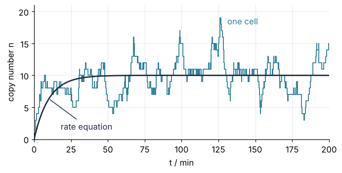
Copy number of one simulated cell against time in minutes, a staircase of single-molecule steps, with the rate-equation curve rising from 0 to 10. The cell runs ahead of the curve early and below it later, and after 50 min wanders between 3 and 19 molecules instead of settling.

The cell does not follow the rate equation even on the way up: at 5 min it already holds 8 molecules where the curve has 3.9, at 30 min only 6 where the curve has 9.5. After 50 min it wanders between 3 and 19, with 349 events in 200 minutes, 1.7 per minute, a little under the 2 per minute of Step 1 because it starts empty. The rate equation describes the average over many cells, not any one of them.

Step 4: Simulate many cells and compare with the Poisson distribution

To measure the spread, simulate 5,000 cells and read each at one time. They start at zero, so read them at 100 min, ten relaxation times, where what is left of the start is \(10\,e^{-10}\), under a thousandth of a molecule. state_at from Step 3 gives each cell's state at that time.

The Fano factor needs an error bar before it can be compared with 1. The standard error \(\sigma/\sqrt{N}\) of The standard error of the mean is for a mean, and the Fano factor is a variance divided by a mean, which has no such simple formula. So split the 5,000 cells into 20 independent groups of 250. That gives 20 measurements of the Fano factor, and the standard error of their mean is the error bar.

N_CELLS, T_READ = 5000, 100.0

def snapshot(stoich, propensities):
    counts = np.empty(N_CELLS, dtype=int)
    for i in range(N_CELLS):
        T, X = gillespie([0], stoich, propensities, T_READ, rng)
        counts[i] = state_at(T, X, T_READ)[0]
    return counts

def fano_with_error(counts, n_groups=20):
    groups = counts.reshape(n_groups, -1)
    fano = groups.var(axis=1, ddof=1) / groups.mean(axis=1)
    return fano.mean(), fano.std(ddof=1) / np.sqrt(n_groups)

counts = snapshot(stoich, propensities)
F, dF = fano_with_error(counts)
print(f"mean {counts.mean():.2f}   std {counts.std(ddof=1):.2f}   Fano {F:.2f} ± {dF:.2f}")
for n in [5, 10, 15, 20]:
    print(f"P({n:2d})  simulated {np.mean(counts == n):.4f}   Poisson {stats.poisson.pmf(n, 10):.4f}")

mean 10.07   std 3.21   Fano 1.02 ± 0.02
P( 5)  simulated 0.0372   Poisson 0.0378
P(10)  simulated 0.1212   Poisson 0.1251
P(15)  simulated 0.0334   Poisson 0.0347
P(20)  simulated 0.0030   Poisson 0.0019

The mean is 10.07 and the standard deviation 3.21, against 10 and \(\sqrt{10} = 3.16\), and the Fano factor is 1.02 ± 0.02, consistent with 1. The probabilities follow the Poisson values to within 0.004. Independent single-molecule events make exactly this much noise between cells, and no more.

Step 5: Average one long trajectory over time

Many cells at one time is what a microscope sees. The alternative is one cell followed for a long time, 100,000 minutes here. For this process the two give the same answer: the average over time equals the average over cells, which is what ergodic means. The event list, however, is not a sample at regular times. Each state must count for as long as it was held, so the weights are the gaps between events, with the end time appended for the last state. The first 50 minutes, five relaxation times, are dropped; five are enough here because what is left of the start shifts a 100,000-minute average by under \(10^{-5}\) molecules.

T_LONG = 100_000.0
T_long, X_long = gillespie([0], stoich, propensities, T_LONG, rng)
n_long = X_long[:, 0]
dt = np.diff(np.append(T_long, T_LONG))      # how long each state was held
keep = T_long >= 50
mean_t = np.average(n_long[keep], weights=dt[keep])
var_t = np.average((n_long[keep] - mean_t) ** 2, weights=dt[keep])
p_t = np.bincount(n_long[keep], weights=dt[keep]) / dt[keep].sum()
print(f"{len(T_long) - 1} events   time-weighted mean {mean_t:.2f}   Fano {var_t / mean_t:.2f}")
print(f"P(10)  time-weighted {p_t[10]:.4f}   Poisson {stats.poisson.pmf(10, 10):.4f}")

200703 events   time-weighted mean 10.07   Fano 1.03
P(10)  time-weighted 0.1220   Poisson 0.1251

One trajectory of 200,703 events gives a time-weighted mean of 10.07 and a Fano factor of 1.03, against 10.07 and 1.02 from 5,000 cells, with a fifth of the events. Leave out the weights and the mean comes out wrong; that is the first pitfall.

Step 6: Make production bursty and measure the Fano factor

Bursts come from the messenger RNA: one mRNA is made, translated several times, and decays. Each translation races against the decay of the mRNA, so the number of proteins from one mRNA is geometric, \(P(B = m) = \frac16 \left(\frac56\right)^m\) for \(m = 0, 1, 2, \dots\), with mean \(b = 5\). At \(k_b = 0.2\) bursts per minute that is still 1 molecule per minute.

The loop needs no change. Bursts of each size are independent events with their own rate, \(k_b P(B = m)\), and that is all a reaction is: a burst of \(m\) molecules is a row of the table with change \(+m\). A burst of size 0 changes nothing and is left out, which is why the rows add up to \(\frac56 \cdot 0.2 = 1/6\) bursts per minute and not 0.2. The table stops at \(m = 120\), where the probability left out is \((5/6)^{121} \approx 3 \times 10^{-10}\).

m = np.arange(1, 121)
p_burst = 1 / (1 + B_MEAN) * (B_MEAN / (1 + B_MEAN)) ** m
rates_burst = K_BURST * p_burst
stoich_burst = np.vstack([m[:, None], [[-1]]])   # 120 burst rows, then loss

def propensities_burst(x):
    return np.append(rates_burst, GAMMA * x[0])

print(f"bursts per minute          {rates_burst.sum():.4f}")
print(f"molecules made per minute  {(rates_burst * m).sum():.4f}")

bursts per minute          0.1667
molecules made per minute  1.0000

The rows make 1.0000 molecule per minute: the same rate equation, with the same steady state of 10.

The theory for this model is a negative binomial distribution (Shahrezaei and Swain, 2008). SciPy's stats.nbinom(r, p) counts the failures before the \(r\)-th success. Here \(r = k_b/\gamma = 2\), the number of bursts in one molecule's mean lifetime, and \(p = 1/(1 + b) = 1/6\). For your own \(k_b\), \(\gamma\), and \(b\) only these two numbers change, and the printed mean \(r(1 - p)/p\) checks them:

nb = stats.nbinom(K_BURST / GAMMA, 1 / (1 + B_MEAN))
print(f"theory: mean {nb.mean():.1f}   std {nb.std():.2f}   Fano {nb.var() / nb.mean():.1f}")

counts_burst = snapshot(stoich_burst, propensities_burst)
F_b, dF_b = fano_with_error(counts_burst)
print(f"simulated: mean {counts_burst.mean():.2f}   std {counts_burst.std(ddof=1):.2f}   Fano {F_b:.2f} ± {dF_b:.2f}")
for n in [0, 5, 10, 20, 30]:
    print(f"P({n:2d})  simulated {np.mean(counts_burst == n):.4f}   negative binomial {nb.pmf(n):.4f}")
print(f"P( 0)  Poisson, for comparison {stats.poisson.pmf(0, 10):.6f}")

theory: mean 10.0   std 7.75   Fano 6.0
simulated: mean 10.19   std 7.85   Fano 6.03 ± 0.14
P( 0)  simulated 0.0278   negative binomial 0.0278
P( 5)  simulated 0.0616   negative binomial 0.0670
P(10)  simulated 0.0482   negative binomial 0.0493
P(20)  simulated 0.0174   negative binomial 0.0152
P(30)  simulated 0.0040   negative binomial 0.0036
P( 0)  Poisson, for comparison 0.000045

The simulated cells have a mean of 10.19, a standard deviation of 7.85 against 7.75, and a Fano factor of 6.03 ± 0.14 against \(1 + b = 6\). The same mean now hides 2.8 % of cells with no protein at all, where the Poisson distribution has 0.0045 %. The figure from the beginning puts the two models side by side:

T_c, X_c = gillespie([0], stoich, propensities, 300, rng)
T_b, X_b = gillespie([0], stoich_burst, propensities_burst, 300, rng)

fig, (ax, ax_h) = plt.subplots(1, 2, figsize=(8, 3.6), sharey=True,
                               gridspec_kw={"width_ratios": [3, 1]})
ax.step(T_c, X_c[:, 0], where="post", color=SECOND, lw=1.2)
ax.step(T_b, X_b[:, 0], where="post", color=ACCENT, lw=1.2)
ax.axhline(K / GAMMA, color=MUTED, lw=1, ls="--")
ax.text(137, 44, "bursty", color=ACCENT)
ax.text(153, 18.5, "one at a time", color=SECOND)
ax.text(303, 10, "k/γ", color=MUTED, va="center")
ax.set(xlabel="t / min", ylabel="copy number n", xlim=(100, 300), ylim=(0, 50))

bins = np.arange(-0.5, 51)
n_axis = np.arange(0, 51)
ax_h.hist(counts, bins=bins, density=True, orientation="horizontal", color=SECOND, alpha=0.35)
ax_h.hist(counts_burst, bins=bins, density=True, orientation="horizontal", color=ACCENT, alpha=0.35)
ax_h.plot(stats.poisson.pmf(n_axis, 10), n_axis, color=INK, lw=1.2)
ax_h.plot(nb.pmf(n_axis), n_axis, color=INK, lw=1.2)
ax_h.text(0.06, 15, f"Fano {F:.2f}", color=SECOND)
ax_h.text(0.03, 30, f"Fano {F_b:.2f}", color=ACCENT)
ax_h.set(xlabel="probability")
plt.show()

Left: copy number against time in minutes, 100 to 300, for one cell per model; the one-at-a-time cell stays near 10, the bursty cell jumps to 48 and decays back. Right: histograms of 5,000 cells per model on the Poisson and negative binomial curves; Fano factors 1.02 and 6.03.

The largest excursion in the window, and how long the bursty cell takes to come back:

window = (T_b >= 100) & (T_b <= 300)
i_peak = np.argmax(np.where(window, X_b[:, 0], -1))
jumps = np.diff(X_b[:, 0])
big = [(T_b[j + 1], jumps[j]) for j in np.flatnonzero((jumps > 15) & window[1:])]
back = np.argmax((T_b > T_b[i_peak]) & (X_b[:, 0] <= 10))
print(f"bursty peak {X_b[i_peak, 0]} at {T_b[i_peak]:.1f} min, after bursts of "
      + ", ".join(f"{size} at {t:.1f} min" for t, size in big))
print(f"back to 10 after {T_b[back] - T_b[i_peak]:.1f} min;   one at a time: n from "
      f"{X_c[T_c >= 100, 0].min()} to {X_c[T_c >= 100, 0].max()}")

bursty peak 48 at 130.7 min, after bursts of 19 at 130.6 min, 23 at 130.7 min
back to 10 after 19.3 min;   one at a time: n from 3 to 16

The bursty cell climbs to 48 in two bursts, of 19 and 23 molecules at 130.6 and 130.7 min, and needs 19.3 minutes to come back down to 10, about two relaxation times, while the other cell stays between 3 and 16. Same rate equation, same mean, six times the variance.

Pitfalls

Averaging over reaction events instead of over time. The arrays from the loop hold one state per event, and it is tempting to take their mean:

T_bl, X_bl = gillespie([0], stoich_burst, propensities_burst, T_LONG, rng)
print(f"mean over events: one at a time {n_long.mean():.2f}   bursty {X_bl[:, 0].mean():.2f}")

mean over events: one at a time 10.58   bursty 15.30

The one-at-a-time cell gives 10.58 instead of 10.07, the bursty one 15.30 instead of 10. The list holds one entry per event, so a state collects entries at its total propensity \(a_0\): the faster it is left, the more entries it gets for each minute the cell spends in it. At high copy numbers loss is fast, so those states are overcounted, and after a burst the cell comes down one molecule at a time, each step an entry, where it went up in a single one. Weight each state by how long it was held, as in Step 5, or read the states at fixed times, as in Step 4.

Counting the transient. A cell started from zero stays below 10 for the first few relaxation times. Average a trajectory over its first 100 minutes from \(t = 0\) and you get about 9.0, the average of the rate-equation curve over that window; read cells at 20 minutes and you get \(10\,(1 - e^{-2}) \approx 8.6\). Both are 10 % or more too low, and both look like reasonable numbers. Start averaging or reading only after several relaxation times \(1/\gamma\): Step 5 drops five, Step 4 waits ten.

A Python loop for large copy numbers. Every event is one pass through the Python loop, and the number of events per minute grows with the copy number: about 2 at 10 molecules, as in Step 3, and about 200 at 1,000. The 5,000 cells of Step 4 already took about a million passes. For proteins in the thousands, switch to tau-leaping (below) or move the loop into compiled code; the algorithm stays the same.

Variations

mRNA and protein. Two columns in stoich, mRNA and protein, and four rows: transcription, mRNA decay, translation, protein loss, with four propensities. The loop of Step 2 runs unchanged, and the geometric bursts of Step 6 come out of it instead of going in.
Tau-leaping. Take a fixed step \(\tau\), draw how often each reaction fired from rng.poisson(a * tau), and apply x = x + firings @ stoich. It is fast for large copy numbers and approximate, and a copy number can go negative when \(\tau\) is too large.
A toggle switch. Two repressors that shut each other off give two stable states and cells that flip between them rarely. A long-time average then no longer matches the snapshot of many cells unless the run covers many flips.
An SIR epidemic in a village of 100. Two rows, infection (\(S - 1\), \(I + 1\)) at rate \(\beta S I / N\) and recovery (\(I - 1\), \(R + 1\)) at rate \(\nu I\). Some outbreaks die out by chance where the rate equation predicts an epidemic.

Cheat sheet

stoich = np.array([[+1], [-1]])                    # one row per reaction, one column per species
a = propensities(x); a0 = a.sum()                  # rates per unit time, and their total
t += rng.exponential(1 / a0)                       # waiting time to the next reaction
j = np.searchsorted(np.cumsum(a), rng.random() * a0, side="right")   # which reaction fires
x = x + stoich[j]                                  # apply it
x_t = X[np.searchsorted(T, t, side="right") - 1]   # state at a fixed time t
dt = np.diff(np.append(T, t_end))                  # time weights for averages over one run
fano = n.var(ddof=1) / n.mean()                    # 1 for Poisson, 1 + b for geometric bursts
# a burst of size m is a row with change +m and rate k_b * P(B = m)