Conjugate gradients and the condition number: why iterations grow as √κ
Afterwards you can explain why conjugate gradients converge, predict how their iterations grow with the condition number, and say what preconditioning changes.
- Field
- Engineering, Physics
- Libraries
matplotlib 3.11.2numpy 2.4.3scipy 1.18.1
py-conjugate-gradient.ipynb, executed with the versions above. The download needs a free account
Run it yourself. In a terminal, this installs exactly the versions above:
pip install numpy==2.4.3 scipy==1.18.1 matplotlib==3.11.2 jupyterlabThe question
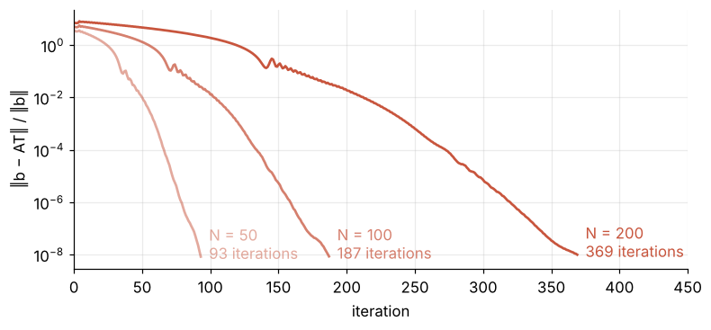
A square plate of side 1 is heated uniformly and its edges are held at temperature 0. The steady temperature obeys −∇²T = q/k, with q the heat produced per unit volume and k the conductivity, and in units of qL²/k the equation is −∇²T = 1. On an N × N grid of interior points the five-point stencil turns it into a linear system A T = b, as in Poisson's equation with scipy.sparse: A is the negated five-point Laplacian, symmetric and positive definite with at most five nonzeros per row, and b is all ones. At N = 1000 there are 10⁶ unknowns, and a dense A would take 10¹² entries of 8 bytes each, 8 TB. Conjugate gradients, CG for short, never need A as a table. They only multiply it by vectors. Here is scipy.sparse.linalg.cg on three grids, with the relative residual ‖b − AT‖/‖b‖ recorded after every iteration until it reaches 10⁻⁸:
Show code
import numpy as np
import scipy.sparse as sp
from scipy.sparse.linalg import cg, LinearOperator, spilu, spsolve_triangular, eigsh, eigs, splu, spsolve
import matplotlib.pyplot as plt

plt.rcParams.update({
    "figure.figsize": (8, 3.4), "figure.dpi": 110,
    "axes.spines.top": False, "axes.spines.right": False,
    "axes.grid": True, "grid.alpha": 0.25,
    "font.size": 11, "lines.linewidth": 1.8,
})
INK, ACCENT, SECOND, MUTED = "#1f2a44", "#c8553d", "#2a7f9e", "#8a8f98"


def laplacian(N):
    """Negated five-point Laplacian on the N x N interior grid of the unit square, edges at 0."""
    h = 1 / (N + 1)
    D = sp.diags_array([-np.ones(N - 1), 2 * np.ones(N), -np.ones(N - 1)], offsets=[-1, 0, 1])
    I = sp.eye_array(N)
    return ((sp.kron(I, D) + sp.kron(D, I)) / h**2).tocsr()


def cg_history(A, b, M=None):
    """CG from x0 = 0 to rtol 1e-8; returns x and the relative residual after each iteration."""
    history = []
    norm_b = np.linalg.norm(b)
    x, info = cg(A, b, rtol=1e-8, maxiter=5000, M=M,
                 callback=lambda xk: history.append(np.linalg.norm(b - A @ xk) / norm_b))
    assert info == 0, "CG did not converge"
    return x, np.array(history)


sizes = [50, 100, 200]
shades = [0.5, 0.75, 1.0]                       # one color, N told apart by alpha
plain = {N: cg_history(laplacian(N), np.ones(N * N)) for N in sizes}

fig, ax = plt.subplots()
for N, a in zip(sizes, shades):
    res = plain[N][1]
    ax.semilogy(np.arange(1, res.size + 1), res, color=ACCENT, alpha=a)    # plain CG is ACCENT in every figure
    ax.text(res.size + 6, 0.6 * res[-1], f"N = {N}\n{res.size} iterations", color=ACCENT, alpha=a, va="bottom")
ax.set(xlabel="iteration", ylabel="‖b − AT‖ / ‖b‖", xlim=(0, 450))
plt.show()

# the center of the plate at N = 200, where it falls between four grid points
N = 200
T_cg = plain[N][0]
T_direct = spsolve(laplacian(N).tocsc(), np.ones(N * N))
center = lambda T: T.reshape(N, N)[N // 2 - 1 : N // 2 + 1, N // 2 - 1 : N // 2 + 1].mean()
m = np.arange(1, 2000, 2)[:, None]              # the exact Fourier series has odd terms only
n = m.T
series = np.sum(16 / np.pi**4 * (-1.0) ** ((m - 1) // 2 + (n - 1) // 2) / (m * n * (m**2 + n**2)))
print(f"center temperature, N = 200:  CG {center(T_cg):.5f}   spsolve {center(T_direct):.5f}"
      f"   exact series {series:.5f}   (units of qL²/k)")
center temperature, N = 200: CG 0.07367 spsolve 0.07367 exact series 0.07367 (units of qL²/k)
The center temperature agrees with a direct solve and with the exact Fourier series to all five digits shown. That part is no surprise. The residual does not fall steadily: it first climbs above 1 and wanders, then drops roughly geometrically, faster toward the end. Each doubling of N doubles the count, 93, 187, 369 iterations.
The less obvious part is why this works at all, and why the count tracks N. CG never looks at an entry of A, yet it finds the 40,000 temperatures of the finest grid with 369 matrix-vector products. The condition number κ of A, the amplification factor of The condition number, grows like 4N²/π² (derived below). So the count grows like √κ, not like κ, which would have quadrupled it per doubling. Whether anything makes it grow more slowly still is the test at the end: the same curves with a preconditioner, and the count against N on log axes.
The idea: walk downhill without undoing earlier steps
Every symmetric positive definite system is a minimization in disguise. Take the energy
Its gradient is Ax − b, the negative of the residual r = b − Ax. The gradient vanishes exactly where Ax = b, and because A is positive definite, f is a bowl with that point x* at its bottom. The residual, which any solver can compute, points downhill.
The simplest way down is steepest descent: from the current x, walk along r until f stops falling, then take the new residual and repeat. Walking until f stops falling is called an exact line search, and for a quadratic it has a closed form: along x + αr the energy is lowest at α = rᵀr / rᵀAr. That costs one product with A per step, the same as one CG iteration.
To compare methods you need a measure of how far from the bottom you are. The height of the bowl above its bottom is
so \(\|e\|_A = \sqrt{e^\mathsf{T} A e}\), the A-norm of the error, says how high up the bowl you still are. CG's guarantee is stated in this norm. A solver cannot compute it without knowing x*, which is why the plate figures show the residual r = −Ae instead; measured relative to their starting values, the two never differ by more than a factor of √κ.
The smallest bowl that shows the trouble is two-dimensional: A = diag(1, κ) and b = 0, so the bottom is at the origin and the valley is √κ times longer than it is wide. Start both methods from (κ, 1) and count the steps until the A-norm error has fallen to 10⁻⁶ of its starting value:
Show code
def descend(kappa, conjugate, tol=1e-6, max_steps=5000):
    """Steepest descent or CG with exact line searches on f = x^T A x / 2, A = diag(1, kappa)."""
    A = np.diag([1.0, kappa])
    x = np.array([kappa, 1.0])
    r = -A @ x
    p = r.copy()
    path, err = [x.copy()], [1.0]
    height0 = np.sqrt(x @ A @ x)
    while err[-1] > tol and len(path) <= max_steps:
        if not conjugate:
            p = r                                   # always straight downhill
        alpha = (r @ r) / (p @ A @ p)
        x = x + alpha * p
        r_new = r - alpha * (A @ p)
        if conjugate:
            p = r_new + (r_new @ r_new) / (r @ r) * p
        r = r_new
        path.append(x.copy())
        err.append(np.sqrt(x @ A @ x) / height0)
    return np.array(path), np.array(err)


fig, axes = plt.subplot_mosaic([["1", "10"], ["100", "100"]], figsize=(8, 5),
                                width_ratios=[1, 1.6], height_ratios=[1.35, 1], layout="constrained")
for kappa in [1, 10, 100]:
    ax = axes[str(kappa)]
    sd_path, sd_err = descend(kappa, conjugate=False)
    cg_path, cg_err = descend(kappa, conjugate=True)
    print(f"κ = {kappa:3d}:  steps to 1e-6,  steepest descent {sd_err.size - 1:3d},  CG {cg_err.size - 1}")
    length, width = 1.1 * np.sqrt(kappa**2 + kappa), 1.1 * np.sqrt(kappa + 1)   # the contour through the start
    x_lo = -length if kappa == 1 else -0.06 * kappa         # the round bowl whole, the valleys from their bottom
    X, Y = np.meshgrid(np.linspace(x_lo, length, 400), np.linspace(-width, width, 200))
    ax.contour(X, Y, 0.5 * (X**2 + kappa * Y**2), levels=np.geomspace(1e-3, 1, 9) * 0.5 * (kappa**2 + kappa),
               colors=MUTED, linewidths=0.7)
    shown = sd_path[:31]                                    # at κ = 100 the zigzag gets dense
    ax.plot(shown[:, 0], shown[:, 1], "-o", color=INK, ms=2.5, lw=1)
    ax.plot(cg_path[:, 0], cg_path[:, 1], "-o", color=ACCENT, ms=4)
    ax.set(xlim=(x_lo, length), ylim=(-width, width), aspect="equal", xlabel="x₁", ylabel="x₂")
    lines = [(f"κ = {kappa}", INK), (f"steepest descent: {sd_err.size - 1}", INK), (f"CG: {cg_err.size - 1}", ACCENT)]
    for row, (label, color) in enumerate(lines):
        ax.annotate(label, (0, 1), xycoords="axes fraction", xytext=(4, -4 - 14 * row), textcoords="offset points",
                    va="top", color=color, bbox=dict(fc="white", ec="none", alpha=0.85, pad=0.5))
plt.show()
κ =   1:  steps to 1e-6,  steepest descent   1,  CG 1
κ =  10:  steps to 1e-6,  steepest descent  69,  CG 2
κ = 100:  steps to 1e-6,  steepest descent 691,  CG 2
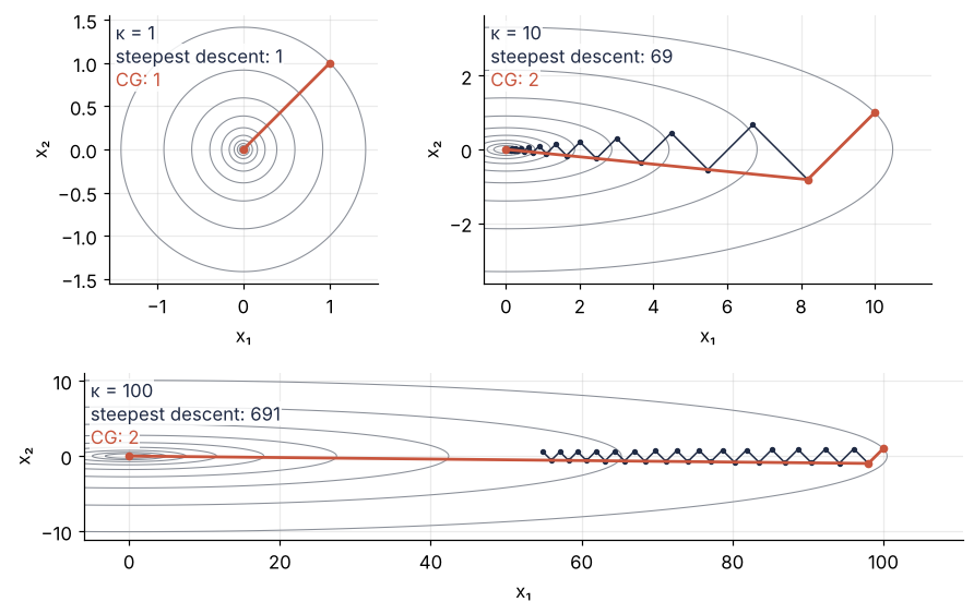
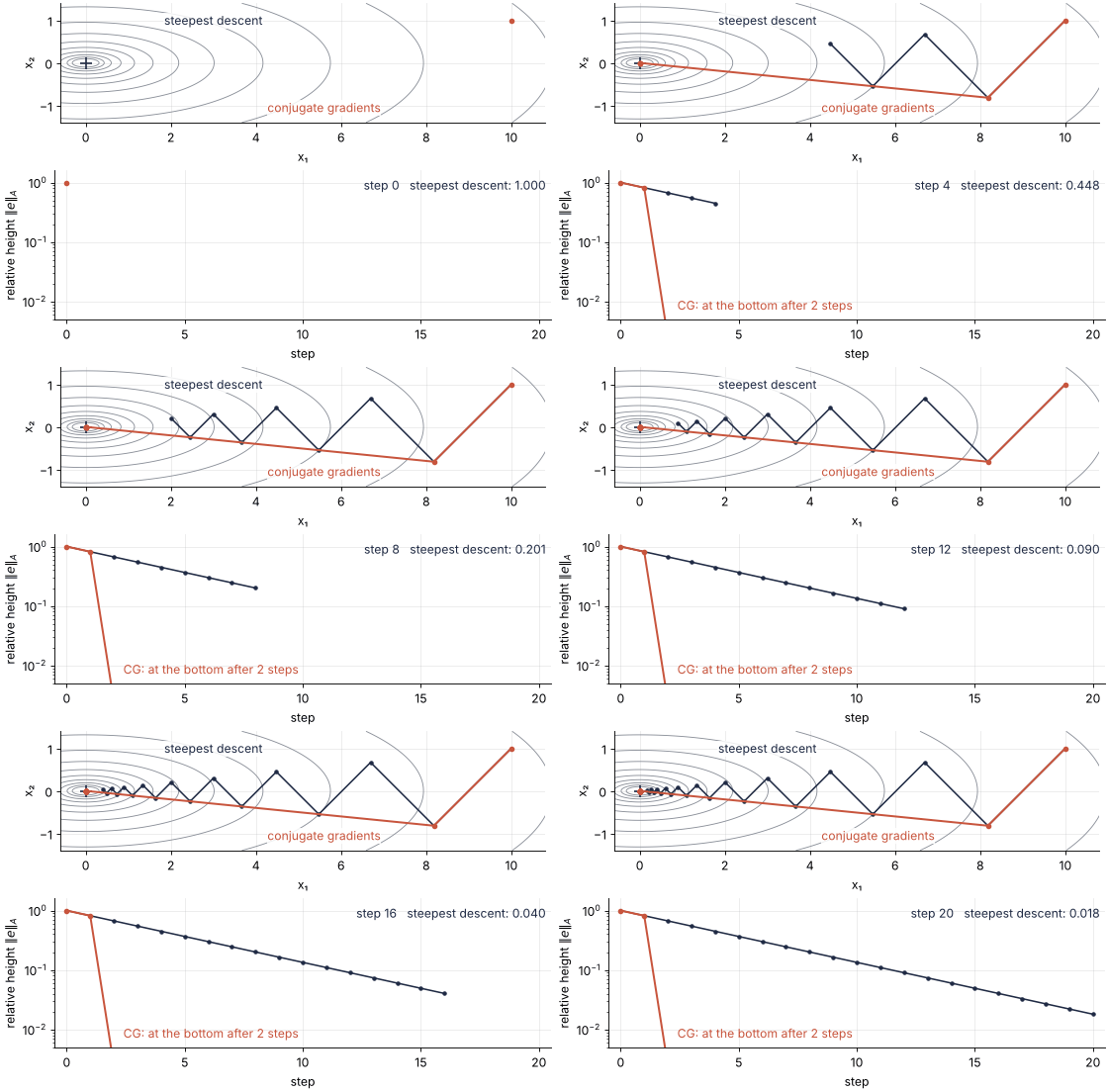
On the round bowl, κ = 1, the residual points straight at the bottom and both methods arrive in one step. At κ = 10 steepest descent needs 69 steps, at κ = 100 it needs 691, of which the figure draws the first 30. CG needs 2 steps in both valleys, however narrow. Here is the race on the κ = 10 valley:
Show code
"""Descent race: steepest descent and conjugate gradients on the same narrow valley.

Renders ../../assets/descent-race.gif for the conjugate-gradient tutorial. The valley is
the energy f(x) = 1/2 x^T A x with A = diag(1, 10), so the bottom is at the origin, and both
methods start from (10, 1). Top: the two paths, drawn one step at a time. Bottom: the height
above the bottom of the bowl, the A-norm of the error, against the step. Run it from any directory:

    python scene.py
"""
from pathlib import Path

import numpy as np
import matplotlib.pyplot as plt
from matplotlib.animation import FuncAnimation, PillowWriter
from PIL import Image

OUT = Path(__file__).resolve().parents[2] / "assets" / "descent-race.gif"
INK, ACCENT, SECOND, MUTED = "#1f2a44", "#c8553d", "#2a7f9e", "#8a8f98"
plt.rcParams.update({"axes.spines.top": False, "axes.spines.right": False,
                     "axes.grid": True, "grid.alpha": 0.25, "font.size": 11})

# ---- data: both methods with exact line searches, as in the tutorial
kappa = 10.0
A = np.diag([1.0, kappa])
STEPS = 20                                                    # steps shown


def descend(conjugate):
    x = np.array([kappa, 1.0])
    r = -A @ x
    p = r.copy()
    path = [x.copy()]
    for _ in range(STEPS):
        if not conjugate:
            p = r                                             # steepest descent: always straight downhill
        if r @ r < 1e-28:                                     # at the bottom: stay there
            path.append(x.copy())
            continue
        alpha = (r @ r) / (p @ A @ p)
        x = x + alpha * p
        r_new = r - alpha * (A @ p)
        if conjugate:
            p = r_new + (r_new @ r_new) / (r @ r) * p
        r = r_new
        path.append(x.copy())
    return np.array(path)


def a_norm(path):
    return np.sqrt(np.einsum("ki,ij,kj->k", path, A, path)) / np.sqrt(path[0] @ A @ path[0])


sd, cg = descend(False), descend(True)
err_sd, err_cg = a_norm(sd), a_norm(cg)
FLOOR = 5e-3                                                  # bottom of the error panel
err_cg = np.maximum(err_cg, FLOOR / 2)                        # after step 2 only rounding: drawn below the floor, off the panel

SUB = 5                                                       # frames per step
HOLD = 12                                                     # frames at the end
frames = np.concatenate([np.linspace(0, STEPS, STEPS * SUB + 1), np.full(HOLD, float(STEPS))])

# ---- figure, drawn once
fig, (ax1, ax2) = plt.subplots(2, 1, figsize=(7, 4.6), dpi=80, height_ratios=[1, 1.25],
                               layout="constrained")
X, Y = np.meshgrid(np.linspace(-0.6, 10.8, 300), np.linspace(-1.4, 1.4, 120))
ax1.contour(X, Y, 0.5 * (X**2 + kappa * Y**2), levels=np.geomspace(0.05, 60, 12),
            colors=MUTED, linewidths=0.8)
ax1.plot(0, 0, "+", color=INK, ms=10, mew=1.5)
(sd_line,) = ax1.plot([], [], "-o", color=INK, ms=3, lw=1.4)
(cg_line,) = ax1.plot([], [], "-o", color=ACCENT, ms=4, lw=1.8)
ax1.set(xlim=(-0.6, 10.8), ylim=(-1.4, 1.4), aspect="equal", xlabel="x₁", ylabel="x₂")
label_box = dict(fc="white", ec="none", alpha=0.85, pad=0.5)  # keeps the contours from crossing the names
ax1.text(3.0, 1.0, "steepest descent", color=INK, ha="center", va="center", bbox=label_box)
ax1.text(5.6, -1.05, "conjugate gradients", color=ACCENT, ha="center", va="center", bbox=label_box)
(sd_err,) = ax2.semilogy([], [], "-o", color=INK, ms=3, lw=1.4)
(cg_err,) = ax2.semilogy([], [], "-o", color=ACCENT, ms=4, lw=1.8)
cg_note = ax2.text(2.4, FLOOR * 1.3, "", color=ACCENT, va="bottom")
step_text = ax2.text(0.99, 0.95, "", transform=ax2.transAxes, ha="right", va="top", color=INK)
ax2.set(xlim=(-0.5, STEPS + 0.5), ylim=(FLOOR, 1.6), xticks=range(0, STEPS + 1, 5),
        xlabel="step", ylabel=r"relative height $\|e\|_A$")


def partial(path, s):
    """The path up to step s, with the current step drawn part of the way."""
    k = int(np.floor(s))
    pts = path[: k + 1]
    if k < STEPS:
        frac = s - k
        pts = np.vstack([pts, path[k] + frac * (path[k + 1] - path[k])])
    return pts


# ---- one frame: a function of the step count alone
def update(s):
    for line, path in [(sd_line, sd), (cg_line, cg)]:
        pts = partial(path, s)
        line.set_data(pts[:, 0], pts[:, 1])
        line.set_markevery(range(int(np.floor(s)) + 1))
    k = int(np.floor(s))
    steps = np.arange(k + 1)
    sd_err.set_data(steps, err_sd[: k + 1])
    cg_err.set_data(steps, err_cg[: k + 1])
    cg_note.set_text("CG: at the bottom after 2 steps" if k >= 2 else "")
    step_text.set_text(f"step {k}   steepest descent: {err_sd[k]:.3f}")


# ---- render, and read back what was written
OUT.parent.mkdir(exist_ok=True)
FuncAnimation(fig, update, frames=frames).save(OUT, writer=PillowWriter(fps=12))
plt.close(fig)
with Image.open(OUT) as im:
    delay = im.info["duration"]
    print(f"{OUT.name}: {im.width} x {im.height} px, {im.n_frames} frames at {delay} ms, "
          f"{im.n_frames * delay / 1000:.1f} s, {OUT.stat().st_size / 1024:,.0f} kB")
Why steepest descent zigzags, and how conjugate directions stop it
An exact line search stops where the path runs along a contour, so the new gradient is perpendicular to the step just taken. In a narrow valley that perpendicular points mostly across the valley, and the next step crosses the floor again, partly undoing what the one before achieved. Steepest descent spends almost every step on the width of the valley and creeps along its length.
CG keeps the line search and changes the direction. Each new direction is A-conjugate to all earlier ones, pᵢᵀApⱼ = 0. In the picture, the first step ends where the path touches a contour ellipse, and the direction conjugate to it runs from that point straight through the center of the ellipse. Minimizing along it does not spoil the minimum already found along the first direction, so nothing is undone. In n dimensions this makes CG exact after n steps, in exact arithmetic, and in two dimensions after 2. On the plate n is 40,000, yet CG was done after 369. Why it gets there so much sooner than n is what the formalization explains.
Preconditioning: make the valley round before walking down it
A preconditioner is a matrix M that resembles A but is cheap to solve with. CG then walks down the valley of M⁻¹A instead of A, and the better M resembles A, the rounder that valley is. On the κ = 100 valley, dividing each equation by its diagonal entry makes the valley round in one move: that is Jacobi preconditioning, M = diag(A). On the plate every diagonal entry is the same 4/h², so Jacobi has nothing to rescale.
Incomplete LU, spilu in SciPy, runs Gaussian elimination on A but throws away every new entry below a drop tolerance. The preconditioner is M = LU. The factors stay almost as sparse as A, here 2.8 times its nonzeros, so applying M⁻¹ to a vector, one triangular solve with L and one with U, costs about as much as three products with A. Its symmetric twin, incomplete Cholesky with M = LLᵀ, is not in SciPy.
SSOR starts from a Gauss-Seidel sweep. The sweep visits the grid points in order and sets each to the value its own equation demands, the average of its four neighbors plus h²/4 times the source, using the neighbors' newest values. Overrelaxation moves each point ω times as far as that, with ω between 1 and 2. A forward sweep followed by a backward one, started from zero, turns a residual into a correction linearly, so the pair is M⁻¹ applied to the residual: two triangular solves. The M behind it is ω/(2 − ω) (D/ω + L) D⁻¹ (D/ω + U), with D the diagonal of A and L and U its strictly lower and upper triangles, and it is symmetric. The best ω depends on the grid, to leading order ω = 2/(1 + sin πh): 1.884 at N = 50 and 1.969 at N = 200.
Formalization
Written out, CG is five updates per iteration, starting from \(x_0 = 0\) and \(r_0 = p_0 = b\):
\(\alpha_k\) is the exact line search, \(\beta_k\) makes the new direction A-conjugate to the old ones. After k steps \(x_k = p(A)\, b\) lies in the Krylov space \(K_k = \mathrm{span}\{b, Ab, \dots, A^{k-1}b\}\), with p of degree k − 1. The start x₀ = 0 has error e₀ = −x*, so b = Ax* = −Ae₀, and the error is \(e_k = x_k - x^* = q_k(A)\, e_0\) with \(q_k(\lambda) = 1 - \lambda p(\lambda)\), a polynomial of degree k and \(q_k(0) = 1\). Because no conjugate step undoes an earlier one, CG picks of all such polynomials the one that makes \(\|e_k\|_A\) smallest.
Only the spectrum matters. Write \(e_0 = \sum_i c_i v_i\) in the orthonormal eigenvectors of A. Since \(A v_i = \lambda_i v_i\), also \(q(A) v_i = q(\lambda_i) v_i\), and
The matrix enters only through where its eigenvalues lie: the error shrinks at least by the smallest maximum of |q(λ)| on [λmin, λmax] that a polynomial can reach. The ratio of the two ends is κ, since for a symmetric positive definite matrix the singular values are the eigenvalues. With two eigenvalues a degree-2 polynomial can vanish at both, which is why CG finished the 2 × 2 valley in 2 steps.
√κ, not κ. Steepest descent picks a new step length every time, so its polynomial has no simple form. A fixed step of 2/(λmin + λmax) along every residual, Richardson iteration, has one: it repeats the degree-1 factor (1 − 2λ/(λmin + λmax))ᵏ, whose largest value on the interval is ((κ − 1)/(κ + 1))ᵏ. Steepest descent does at least as well per step, and from the start (κ, 1) used in the valleys above exactly as well. CG may place all k roots freely, and the best placement is a Chebyshev polynomial. \(T_k(x) = \cos(k \arccos x)\) is a polynomial of degree k in disguise that wiggles between −1 and +1 on [−1, 1] with k + 1 peaks of equal height. Squeezed onto [λmin, λmax] and divided by its value at λ = 0, it has the smallest maximum there that any polynomial with q(0) = 1 can have. Here are both at k = 10 on [1, 100]:
Show code
k, lam_min, lam_max = 10, 1.0, 100.0
lam = np.linspace(0, lam_max, 4001)
repeated = (1 - 2 * lam / (lam_min + lam_max)) ** k
T_k = lambda z: np.polynomial.chebyshev.chebval(z, [0] * k + [1])
scale = lambda l: (lam_max + lam_min - 2 * l) / (lam_max - lam_min)     # [λmin, λmax] onto [−1, 1]
chebyshev = T_k(scale(lam)) / T_k(scale(0.0))
inside = lam >= lam_min

fig, ax = plt.subplots(figsize=(8, 3))
ax.plot(lam, repeated, color=INK)
ax.plot(lam, chebyshev, color=ACCENT)
ax.text(6, 0.55, "fixed step, one factor ten times", color=INK, va="center")
ax.text(50, -0.37, "scaled Chebyshev polynomial", color=ACCENT, ha="center", va="center")
ax.text(1.8, -0.37, "λmin", color=MUTED, va="center")
for curve, color in [(repeated, INK), (chebyshev, ACCENT)]:
    top = np.abs(curve[inside]).max()
    ax.axhline(top, color=MUTED, ls="--", lw=1)
    ax.text(50, top + 0.02, f"max {top:.2f}", color=color, ha="center", va="bottom")
ax.axhline(-np.abs(chebyshev[inside]).max(), color=MUTED, ls="--", lw=1)
ax.axvline(lam_min, color=MUTED, ls="--", lw=1)
ax.set(xlabel="λ", ylabel="q(λ)", xlim=(0, lam_max), ylim=(-0.45, 1.05))
plt.show()
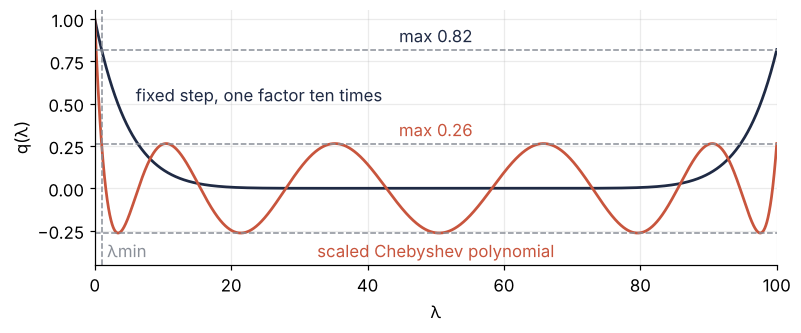
After ten products with A, the fixed step reaches 0.82 and Chebyshev only 0.26, in eleven equal peaks.
That maximum is at most \(2\left((\sqrt\kappa - 1)/(\sqrt\kappa + 1)\right)^k\), and for large κ the ratio is about \(e^{-2/\sqrt\kappa}\), so the bound reaches a tolerance ε after
iterations. Steepest descent needs at most ½κ ln(1/ε), the 691 steps of the κ = 100 valley. On the plate the eigenvalues are (4/h²)(sin²(iπh/2) + sin²(jπh/2)), where i and j, from 1 to N, count the half-waves of a mode across the plate in x and in y: i = j = 1 is the smoothest mode, with the smallest eigenvalue, i = j = N the most wiggly. So κ = cot²(πh/2) ≈ 4(N + 1)²/π², and eigsh confirms both ends at N = 50:
Show code
A = laplacian(50)
h = 1 / 51
# a start vector of all ones would see only the modes with odd i and j; a seeded random one sees all
v0 = np.random.default_rng(1).standard_normal(2500)
ends = np.sort(np.concatenate([eigsh(A, k=1, which="LA", v0=v0, return_eigenvectors=False),
                               eigsh(A, k=1, sigma=0, v0=v0, return_eigenvectors=False)]))
formula = 4 / h**2 * 2 * np.sin(np.array([1, 50]) * np.pi * h / 2) ** 2
print(f"N = 50:  λmin {ends[0]:.4f} (formula {formula[0]:.4f}),  λmax {ends[1]:.2f} (formula {formula[1]:.2f})\n")

print("   N     κ = cot²(πh/2)   4(N+1)²/π²   bound ½√κ·ln(2/ε)   CG measured")
for N in sizes:
    h = 1 / (N + 1)
    kappa = 1 / np.tan(np.pi * h / 2) ** 2
    bound = 0.5 * np.sqrt(kappa) * np.log(2 / 1e-8)
    print(f"{N:4d}   {kappa:14.0f}   {4 * (N + 1)**2 / np.pi**2:10.0f}   {bound:17.0f}   {plain[N][1].size:11d}")
N = 50:  λmin 19.7330 (formula 19.7330),  λmax 20788.27 (formula 20788.27)

   N     κ = cot²(πh/2)   4(N+1)²/π²   bound ½√κ·ln(2/ε)   CG measured
  50             1053         1054                 310            93
 100             4134         4134                 614           187
 200            16373        16374                1223           369
Doubling N quadruples κ and doubles the count. The bound gives 310, 614, and 1223, 3.3 times the measured 93, 187, and 369, because it is a worst case over every b. A right-hand side of all ones excites only the modes with odd i and j, and CG speeds up once its polynomial has put roots near the extreme eigenvalues. What carries over is the growth law.
A preconditioner changes the spectrum. Preconditioned CG applies M⁻¹ to the residual once per iteration, and that action, not M, is what cg takes as its M argument. M⁻¹A is not symmetric, but (M⁻¹Ax)ᵀMy = xᵀAy is symmetric in x and y: measured with xᵀMy in place of the dot product, M⁻¹A behaves like a symmetric positive definite matrix. CG runs unchanged in that product, and κ(M⁻¹A) is the ratio of its largest to its smallest eigenvalue. Jacobi's M is a multiple of the identity: nothing changes. Incomplete LU copies A well over a few grid cells, the scale of the wiggly modes, but not the smoothest mode spanning the plate: κ(M⁻¹A) shrinks by a constant factor and still grows like N², and the count like N. SSOR's ω is tuned to h and lifts the smooth end too. A classical result for this model problem (Axelsson and Barker; Barrett et al., Templates) is that κ(M⁻¹A) then grows only like 1/h ∝ N, so the iterations should grow like √N, half the slope.
See it in code
Show code
def ssor_preconditioner(A, h):
    """M⁻¹ for SSOR with the optimal ω, from two triangular solves; also M itself, for eigsh."""
    omega = 2 / (1 + np.sin(np.pi * h))
    d = A.diagonal()
    lower = (sp.tril(A, -1) + sp.diags_array(d / omega)).tocsr()       # D/ω + L
    upper = (sp.triu(A, 1) + sp.diags_array(d / omega)).tocsr()        # D/ω + U
    def solve(v):
        y = spsolve_triangular(lower, v, lower=True)
        return spsolve_triangular(upper, (2 - omega) / omega * d * y, lower=False)
    M = (omega / (2 - omega) * lower @ sp.diags_array(1 / d) @ upper).tocsc()
    return LinearOperator(A.shape, matvec=solve), M, omega


counts, kappas, ssor_history = {}, {}, {}
for N in sizes:
    A, b, h = laplacian(N), np.ones(N * N), 1 / (N + 1)
    v0 = np.random.default_rng(1).standard_normal(N * N)                # seeded ARPACK start: same run every time
    jacobi = sp.diags_array(1 / A.diagonal())
    M_ssor_inv, M_ssor, omega = ssor_preconditioner(A, h)
    ilu = spilu(A.tocsc(), drop_tol=1e-2, fill_factor=20, permc_spec="NATURAL")   # default ordering breaks symmetry
    M_ilu_inv = LinearOperator(A.shape, matvec=ilu.solve)
    ssor_history[N] = cg_history(A, b, M_ssor_inv)[1]
    counts[N] = dict(none=plain[N][1].size, jacobi=cg_history(A, b, jacobi)[1].size,
                     ilu=cg_history(A, b, M_ilu_inv)[1].size, ssor=ssor_history[N].size)
    # κ(M⁻¹A) for SSOR from the symmetric pencil (A, M)
    top = eigsh(A, k=1, M=M_ssor, which="LA", v0=v0, return_eigenvectors=False)[0]
    bottom = eigsh(A, k=1, M=M_ssor, sigma=0, v0=v0, return_eigenvectors=False)[0]
    # κ(M⁻¹A) for ILU: largest eigenvalue of M⁻¹A, and smallest as 1 / largest of A⁻¹M
    assert (ilu.perm_r == np.arange(N * N)).all() and (ilu.perm_c == np.arange(N * N)).all()
    LU, A_lu = (ilu.L @ ilu.U).tocsr(), splu(A.tocsc())
    ilu_top = eigs(LinearOperator(A.shape, matvec=lambda v: ilu.solve(A @ v)), k=1, v0=v0,
                   return_eigenvectors=False)[0].real
    ilu_inv_bottom = eigs(LinearOperator(A.shape, matvec=lambda v: A_lu.solve(LU @ v)), k=1, v0=v0,
                          return_eigenvectors=False)[0].real
    kappas[N] = dict(ssor=top / bottom, ilu=ilu_top * ilu_inv_bottom, omega=omega,
                     fill=(ilu.L.nnz + ilu.U.nnz) / A.nnz)

print("                iterations to 1e-8                 κ(M⁻¹A)")
print("   N    none  Jacobi  ILU  SSOR      ILU    SSOR    ω      ILU fill   SSOR bound")
for N in sizes:
    c, q = counts[N], kappas[N]
    print(f"{N:4d}   {c['none']:5d} {c['jacobi']:6d} {c['ilu']:5d} {c['ssor']:5d}   {q['ilu']:7.1f} {q['ssor']:6.1f}"
          f"   {q['omega']:.3f}   {q['fill']:6.2f}   {0.5 * np.sqrt(q['ssor']) * np.log(2 / 1e-8):9.0f}")

# the same incomplete LU with SciPy's default column ordering, which leaves M unsymmetric
A, b = laplacian(200), np.ones(200 * 200)
ilu_default = spilu(A.tocsc(), drop_tol=1e-2, fill_factor=20)            # default permc_spec="COLAMD"
x, info = cg(A, b, rtol=1e-8, maxiter=500, M=LinearOperator(A.shape, matvec=ilu_default.solve))
print(f"\nN = 200, ILU with default ordering: fill {(ilu_default.L.nnz + ilu_default.U.nnz) / A.nnz:.2f}, "
      f"residual after 500 iterations {np.linalg.norm(b - A @ x) / np.linalg.norm(b):.1e}")

fig, (ax_res, ax_n) = plt.subplots(1, 2, figsize=(8, 3.6))
for N, a in zip(sizes, shades):
    for res, color in [(plain[N][1], ACCENT), (ssor_history[N], SECOND)]:   # plain CG red, preconditioned blue
        ax_res.semilogy(np.arange(1, res.size + 1), res, color=color, alpha=a)
ax_res.text(225, 1e-6, "none", color=ACCENT)                           # between the N = 100 and 200 curves
ax_res.text(46, 2e-9, "SSOR", color=SECOND, ha="center", va="center")   # under the three SSOR ends
ax_res.set(xlabel="iteration", ylabel="‖b − AT‖ / ‖b‖", xlim=(0, 380),
           ylim=(8e-10, None), yticks=10.0 ** np.arange(-8, 1, 2))   # decades as in the first figure
N_arr = np.array(sizes)
for key, color, marker, label, nudge in [("none", ACCENT, "o", "none", 1.0), ("ilu", SECOND, "s", "incomplete LU", 1.1),
                                        ("ssor", SECOND, "o", "SSOR", 0.9)]:
    ax_n.loglog(N_arr, [counts[N][key] for N in sizes], "-", marker=marker, color=color, ms=6,
                mfc="white" if key == "ilu" else color, mew=1.5)
    ax_n.text(215, nudge * counts[200][key], label, color=color, va="center")   # at the right end, ILU and SSOR nudged apart
ax_n.loglog(N_arr, 1.4 * N_arr, ls="--", lw=1, color=MUTED)
ax_n.loglog(N_arr, 2.2 * np.sqrt(N_arr), ls="--", lw=1, color=MUTED)
ax_n.text(215, 1.4 * 200, "∝ N", color=MUTED, va="center")
ax_n.text(215, 2.2 * np.sqrt(200), "∝ √N", color=MUTED, va="center")
ax_n.set(xlabel="N, grid points per side", ylabel="iterations", xlim=(42, 400),
         xticks=sizes, xticklabels=sizes, yticks=[20, 50, 100, 200, 400], yticklabels=[20, 50, 100, 200, 400])
ax_n.minorticks_off()
fig.tight_layout()
plt.show()
                iterations to 1e-8                 κ(M⁻¹A)
   N    none  Jacobi  ILU  SSOR      ILU    SSOR    ω      ILU fill   SSOR bound
  50      93     93    23    30      10.9   13.0   1.884     2.74          34
 100     187    187    40    43      40.6   25.3   1.940     2.77          48
 200     369    369    76    63     158.7   50.0   1.969     2.78          68

N = 200, ILU with default ordering: fill 4.65, residual after 500 iterations 1.2e-03
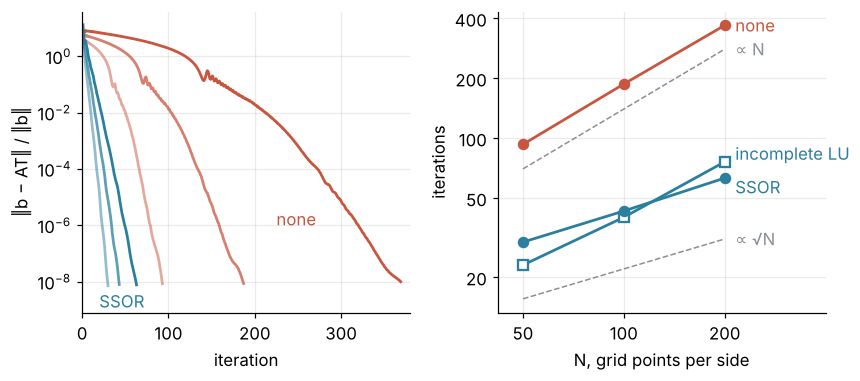
Jacobi gives the counts of no preconditioner, as predicted. Incomplete LU cuts them to 23, 40, and 76, but its κ quadruples with each doubling of N, from 10.9 to 40.6 to 158.7, so the counts still double and the slope stays 1. SSOR's κ only doubles, from 13.0 to 25.3 to 50.0, and its counts of 30, 43, and 63 grow by factors of 1.4 and 1.5 per doubling: the slope of ½ the prediction asked for. For SSOR the bound gives 34, 48, and 68, close to the measurement this time. At N = 200 SSOR needs 63 iterations where plain CG needs 369. Incomplete LU is ahead on the coarse grid, and SSOR overtakes it between N = 100 and 200: for a fine grid, pick the preconditioner by its slope, not by its count on a small test.
One setting decides whether incomplete LU works at all. SciPy's default reorders the columns, which is meant to keep L and U sparse, and leaves M unsymmetric. The last line of the output is that run on the N = 200 plate: after 500 iterations the residual is still at 1.2 × 10⁻³, where CG with no preconditioner at all converges in 369. The reordering does not even save memory here, 4.65 times the nonzeros of A against 2.8 with permc_spec="NATURAL", which keeps M symmetric enough.
Where it shows up
- Structural mechanics. A finite element model of a bridge or a machine part gives a stiffness matrix that is symmetric positive definite once the supports are fixed, and with millions of displacements it is solved with preconditioned CG once a direct factorization runs out of memory. The membrane of scikit-fem from the ground up is a small instance of the same system, solved there directly.
- Fluid dynamics. An incompressible flow solver keeps the velocity free of divergence by solving a Poisson equation for the pressure at every time step, the plate's equation on a far larger grid. OpenFOAM's usual setting for it is the
PCGsolver with theDICpreconditioner, diagonal incomplete Cholesky. - Lattice QCD. Simulations of quarks and gluons solve systems with D†D, where D is the lattice Dirac operator, the sparse matrix that couples the quark field at each site to its neighbors. CG on these normal equations takes most of the machine time of such a simulation.
- Tomography. Reconstructing a CT slice from its projections is a least-squares problem, and CGLS solves it by running CG on the normal equations without ever forming the product of the projection matrix with its transpose. CT reconstruction with scikit-image iterates with SART, another iterative method for the same problem.
- Gaussian processes and kriging. Gaussian-process regression solves with the covariance matrix of the observations plus the noise, which is symmetric positive definite, and at a few hundred thousand points that solve is done with preconditioned CG instead of a Cholesky factorization. Kriging with PyKrige builds a system of the same kind for forty wells, small enough to solve directly.
- Optimization. Newton's method needs a solve with the Hessian at every step, and
scipy.optimize.minimize(method="Newton-CG")does it inexactly with a few CG iterations, which need only products of the Hessian with vectors. Minimization with scipy.optimize.minimize compares its relatives BFGS and L-BFGS-B on a seven-atom cluster.
In every case the cost is about √κ products with a matrix, and the lever is a preconditioner that changes how κ grows with the size of the problem.
Further reading
- The SciPy reference for
cg,LinearOperator,spilu, andspsolve_triangular. - Shewchuk, "An Introduction to the Conjugate Gradient Method Without the Agonizing Pain" (1994), for the geometry of CG and the Chebyshev bound at this level, with many pictures.
- Saad, Iterative Methods for Sparse Linear Systems, 2nd ed. (SIAM, 2003), for SSOR, incomplete factorizations, and their analysis.
- Related tutorials on this site: The condition number: how many digits a linear solve can lose; Poisson's equation with scipy.sparse: two plates in a grounded box; Sparse eigenvalues with scipy.sparse.linalg.eigsh: the tones of a drum; Solve a linear system with NumPy: the currents in a resistor network, the dense direct solve that works for a network and not for 10⁶ unknowns; Matplotlib animation with FuncAnimation: a probe sweep as a small GIF, how an animation like the one above is built.
- Download the notebook. It was executed with the library versions in the header.