Hamiltonian Monte Carlo: why gradients beat a random walk in 100 dimensions
Afterwards you can explain how Hamiltonian Monte Carlo uses gradients and leapfrog steps to move far, tune its step size and path length, and spot a divergence.
- Field
- Biology, Mathematics, Physics
- Libraries
emcee 3.1.6matplotlib 3.11.2numpy 2.4.3
py-hamiltonian-monte-carlo.ipynb, executed with the versions above. The download needs a free account
Run it yourself. In a terminal, this installs exactly the versions above:
pip install emcee==3.1.6 numpy==2.4.3 matplotlib==3.11.2 jupyterlabThe question
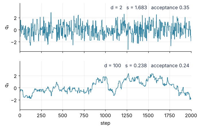
Random-walk Metropolis is the plainest Markov chain Monte Carlo sampler, and the one Hamiltonian Monte Carlo was built to beat. From the current point \(q\) it proposes \(q' = q + s\,\xi\), with \(\xi\) a vector of standard normal numbers and \(s\) the step, and accepts the move with probability \(\min(1, \pi(q')/\pi(q))\), where \(\pi(q)\) is the posterior density. It is the same kind of acceptance test that emcee's stretch move makes. Run it on a standard Gaussian in 2 and in 100 dimensions, each with the textbook step \(s = 2.38/\sqrt d\), and follow the first coordinate for 2,000 steps:
Show code
import math
import numpy as np
import matplotlib.pyplot as plt
from emcee.autocorr import integrated_time

plt.rcParams.update({
    "figure.figsize": (7, 3.6), "figure.dpi": 110,
    "axes.spines.top": False, "axes.spines.right": False,
    "axes.grid": True, "grid.alpha": 0.25,
    "font.size": 11, "lines.linewidth": 1.8,
})
INK, ACCENT, SECOND, MUTED = "#1f2a44", "#c8553d", "#2a7f9e", "#8a8f98"
rng = np.random.default_rng(313)        # one generator for every run below, always in this order


def rwm(log_pi, q0, s, n, rng, thin=1, block=10_000):
    """Random-walk Metropolis: n proposals of step s; keeps every thin-th state."""
    q = np.array(q0, float)
    lp = log_pi(q)
    chain, n_acc = np.empty((n // thin, q.size)), 0
    for start in range(0, n, block):     # noise drawn in blocks, so a long run never holds it all
        m = min(block, n - start)
        xi, log_u = rng.standard_normal((m, q.size)), np.log(rng.random(m))
        for k in range(m):
            q_new = q + s * xi[k]
            lp_new = log_pi(q_new)
            if log_u[k] < lp_new - lp:
                q, lp, n_acc = q_new, lp_new, n_acc + 1
            if (start + k + 1) % thin == 0:
                chain[(start + k) // thin] = q
    return chain, n_acc / n


def leapfrog(q, p, grad, eps, L, U, grad_U, max_dH=np.inf):
    """L leapfrog steps from (q, p), with grad = ∇U(q). Returns the path, H along it, and the end state."""
    path, H = [q], [U(q) + 0.5 * p @ p]
    for _ in range(L):
        p = p - 0.5 * eps * grad
        q = q + eps * p
        grad = grad_U(q)                 # one gradient per step: the next half kick reuses it
        p = p - 0.5 * eps * grad
        path.append(q)
        H.append(U(q) + 0.5 * p @ p)
        if not H[-1] - H[0] <= max_dH:   # diverged (or overflowed to nan): stop, as Stan does
            break
    return np.array(path), np.array(H), p, grad


def hmc(U, grad_U, q0, eps, L_range, n, rng, max_dH=1000.0, keep_paths=False):
    """n HMC iterations, L drawn uniformly from L_range. Counts gradients and divergent trajectories."""
    q = np.array(q0, float)
    grad = grad_U(q)
    chain, work, dH = np.empty((n, q.size)), np.empty(n, int), np.empty(n)
    divergent, paths, n_acc, n_grad = np.zeros(n, bool), [], 0, 0
    for i in range(n):
        p = rng.standard_normal(q.size)
        L = rng.integers(L_range[0], L_range[1] + 1)
        path, H, _, grad_end = leapfrog(q, p, grad, eps, L, U, grad_U, max_dH)
        n_grad += len(path) - 1
        dH[i] = H[-1] - H[0]
        divergent[i] = len(path) - 1 < L or not np.isfinite(dH[i])
        if not divergent[i] and np.log(rng.random()) < -dH[i]:
            q, grad, n_acc = path[-1], grad_end, n_acc + 1
        chain[i], work[i] = q, n_grad
        if keep_paths:
            paths.append((path, H))
    return dict(chain=chain, acc=n_acc / n, work=work, dH=dH, divergent=divergent, paths=paths)


# The question: random-walk Metropolis on a standard Gaussian, textbook step 2.38 / sqrt(d)
runs = {}
for d in [2, 10, 100]:
    s = 2.38 / math.sqrt(d)
    chain, acc = rwm(lambda q: -0.5 * q @ q, rng.standard_normal(d), s, 50_000, rng)
    tau = integrated_time(chain[:, None, :1], quiet=True)[0]
    runs[d] = (s, acc, tau, chain[:, 0])

fig, axes = plt.subplots(2, 1, figsize=(7, 4.4), sharex=True, sharey=True)
for ax, d in zip(axes, [2, 100]):
    s, acc, tau, q1 = runs[d]
    ax.plot(q1[:2000], color=SECOND, lw=1)
    ax.text(0.99, 0.97, f"d = {d}   s = {s:.3f}   acceptance {acc:.2f}", transform=ax.transAxes,
            ha="right", va="top", color=INK)
    ax.set(ylabel="q₁", ylim=(-3.6, 4.4), yticks=[-2, 0, 2])
axes[-1].set(xlabel="step", xlim=(0, 2000))
plt.show()

print("    d   step s   acceptance   τ / proposals")
for d, (s, acc, tau, _) in runs.items():
    print(f"  {d:3d}   {s:6.3f}   {acc:10.3f}   {tau:13.1f}")
    d   step s   acceptance   τ / proposals
    2    1.683        0.352             7.3
   10    0.753        0.263            29.5
  100    0.238        0.242           338.0
Two things are obvious. The acceptance falls from 0.352 in two dimensions toward 0.234, the value theory predicts for this step, which is the best step on this target once the dimension is large (Roberts, Gelman, and Gilks 1997). And the step shrinks as \(1/\sqrt d\), because the change in \(\log\pi\) is a sum over \(d\) coordinates: 0.238 in each of 100 coordinates is already a jump of 2.38, and a longer jump would almost never be accepted.
The price is the autocorrelation time τ, the number of proposals per independent draw: 7.3 in two dimensions, 338 in a hundred. A chain of \(N\) proposals is therefore worth \(N/\tau\) independent draws, its effective sample size (ESS). The walk moves 0.238 per coordinate on each step it takes, and the acceptance says it takes a step on 0.242 of its proposals, so it covers a mean squared distance of \(0.238^2 \times 0.242 = 0.0137\) per proposal. To wander across the bulk of the distribution, two standard deviations, takes \(2^2/0.0137 \approx 290\) proposals, close to the measured τ. That is diffusion, and diffusion is slow.
How can a sampler take steps of several standard deviations in 100 dimensions and still have them accepted? The random walk ignores something the posterior can tell it at every point: which way the density rises.
The idea: let the parameters roll
Turn the posterior into a landscape. Define the potential energy \(U(q) = -\log\pi(q)\): where the posterior is high, \(U\) is low, so its peak becomes the bottom of a valley and \(-\nabla U\) is a force that points toward more probable parameters. Now treat \(q\) as the position of a ball, give it a random kick, a momentum \(p\) drawn from a standard normal distribution, and let it roll without friction for a while. It runs down into the valley and up the far side until its kinetic energy is spent, which is far from where it started. Then kick it again, in a new direction and with a new strength. Because each kick has its own size, each roll runs at its own energy, some low in the valley and some high on its walls, and over many kicks the ball visits the whole posterior. Kick, roll, accept or reject the end point, kick again: that is Hamiltonian Monte Carlo (HMC).
Here is a target where the difference shows, a banana: \(x\) standard normal and \(y\), given \(x\), normal around \(x^2 - 1\) with standard deviation 0.4. Both samplers get 1,000 units of work. For the random walk a unit is one evaluation of the density, for HMC one evaluation of its gradient, which costs a small constant multiple of the density on a general model and exactly as much on the Gaussian later, so HMC gets no free work. The walk spends its budget on 1,000 proposals of step 0.4. HMC spends it on 40 rolls, each computed in 25 time steps of 0.08:
Show code
B = 0.4                                   # width of the banana across its ridge


def U_banana(q):
    x, y = q
    return 0.5 * x**2 + 0.5 * ((y - x**2 + 1) / B) ** 2


def grad_banana(q):
    x, y = q
    r = (y - x**2 + 1) / B**2
    return np.array([x - 2 * x * r, r])


start = np.array([0.0, -1.0])             # the bottom of the valley
rw_chain, rw_acc = rwm(lambda q: -U_banana(q), start, 0.4, 1000, rng)
banana = hmc(U_banana, grad_banana, start, 0.08, (25, 25), 40, rng, keep_paths=True)

xg, yg = np.meshgrid(np.linspace(-3, 3, 300), np.linspace(-2.6, 4, 300))
log_density = -np.array([U_banana((x, y)) for x, y in zip(xg.ravel(), yg.ravel())]).reshape(xg.shape)
fig, axes = plt.subplots(1, 2, figsize=(7, 3.6), sharex=True, sharey=True, layout="constrained")
for ax in axes:
    ax.contour(xg, yg, log_density, levels=[-4.5, -2, -0.5], colors=MUTED, linewidths=1,
               linestyles="solid")
    ax.set(aspect="equal", xlabel="x", xlim=(-3, 3), ylim=(-2.4, 4))
axes[0].plot(*rw_chain.T, "-o", color=SECOND, lw=0.5, ms=2.5)
axes[0].text(0.5, 0.98, f"random walk\n{len(rw_chain):,} evaluations\nacceptance {rw_acc:.2f}",
             transform=axes[0].transAxes, ha="center", va="top", color=INK)
for path, _ in banana["paths"]:
    axes[1].plot(*path.T, color=ACCENT, lw=0.8, alpha=0.35)
axes[1].plot(*banana["chain"].T, "o", color=ACCENT, ms=5)
axes[1].text(0.5, 0.98, f"HMC\n{banana['work'][-1]:,} gradients\nacceptance {banana['acc']:.2f}",
             transform=axes[1].transAxes, ha="center", va="top", color=INK)
axes[0].set_ylabel("y")
plt.show()
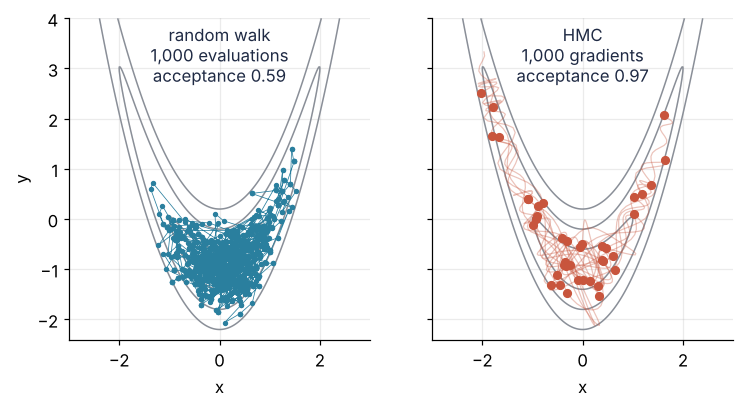
The walk accepts 0.59 of its proposals, and its 1,000 points stay in the bend of the banana, below y = 1.5 on both arms. HMC accepts 0.97, and its 40 points spread up both arms. Every faint line between them is one roll, curving along the banana instead of cutting across it.
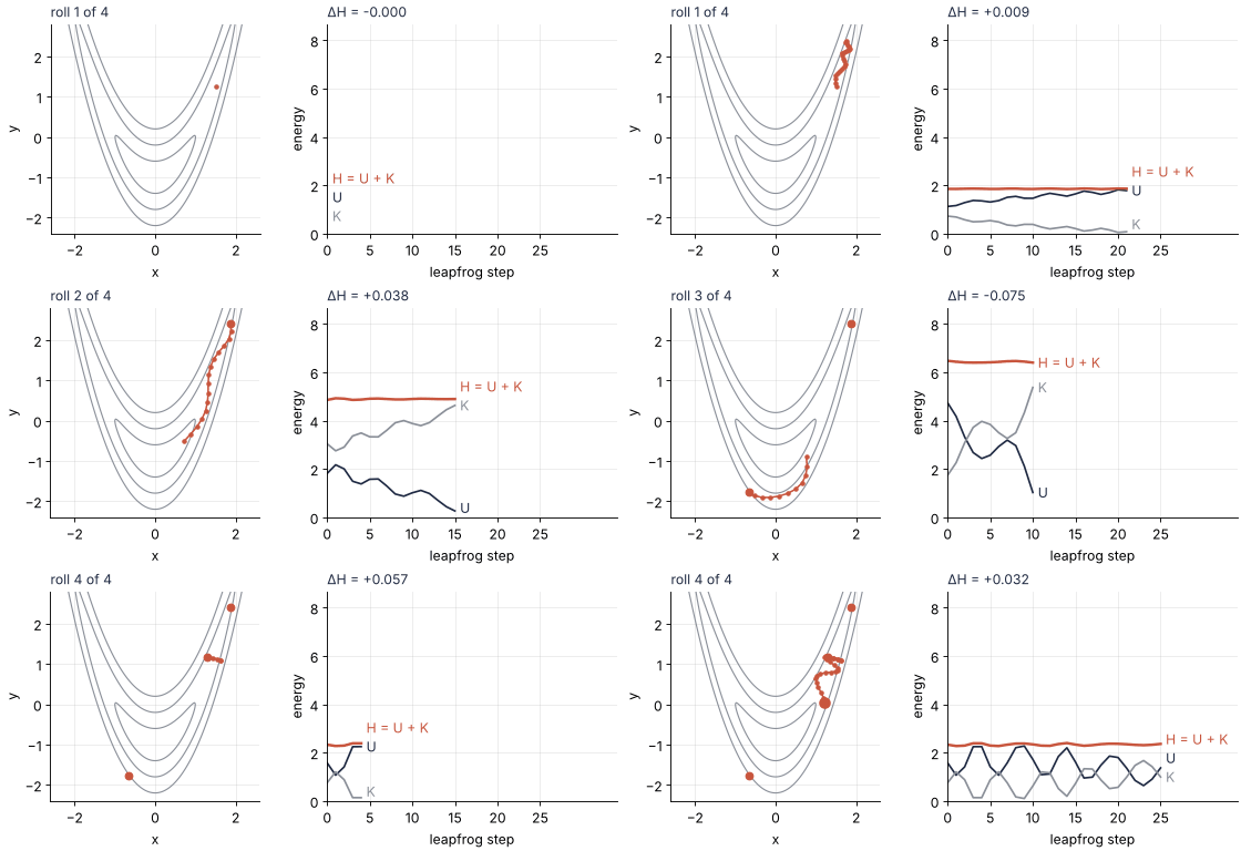
Here are four rolls on the same banana, one time step per frame, with the energies beside them:
Show code
"""Four HMC rolls on the banana, one leapfrog step per frame.

Renders ../../assets/banana-trajectories.gif for the Hamiltonian Monte Carlo tutorial. The target
is x standard normal and y, given x, normal around x^2 - 1 with standard deviation 0.4. Left: the
banana, the current roll, and the samples kept so far. Right: potential energy U, kinetic energy K,
and their sum H along the current roll, each named at its moving line end. Run it from any directory:

    python scene.py
"""
from pathlib import Path

import numpy as np
import matplotlib.pyplot as plt
from matplotlib.animation import FuncAnimation, PillowWriter
from PIL import Image

OUT = Path(__file__).resolve().parents[2] / "assets" / "banana-trajectories.gif"
INK, ACCENT, SECOND, MUTED = "#1f2a44", "#c8553d", "#2a7f9e", "#8a8f98"
plt.rcParams.update({"axes.spines.top": False, "axes.spines.right": False,
                     "axes.grid": True, "grid.alpha": 0.25, "font.size": 11})

# ---- the rolls: the tutorial's banana, step 0.08, 25 steps per roll
B, EPS, STEPS, ROLLS = 0.4, 0.08, 25, 4


def U(q):
    x, y = q
    return 0.5 * x**2 + 0.5 * ((y - x**2 + 1) / B) ** 2


def grad_U(q):
    x, y = q
    r = (y - x**2 + 1) / B**2
    return np.array([x - 2 * x * r, r])


rng = np.random.default_rng(313)
q = np.array([1.5, 1.25])                                     # on the ridge, up the right arm
rolls = []                                                    # (positions, U, K, accepted) per roll
for _ in range(ROLLS):
    p = rng.standard_normal(2)
    path, Us, Ks = [q], [U(q)], [0.5 * p @ p]
    qn = q
    for _ in range(STEPS):                                    # half kick, drift, half kick
        p = p - 0.5 * EPS * grad_U(qn)
        qn = qn + EPS * p
        p = p - 0.5 * EPS * grad_U(qn)
        path.append(qn); Us.append(U(qn)); Ks.append(0.5 * p @ p)
    Us, Ks = np.array(Us), np.array(Ks)
    accepted = np.log(rng.random()) < -((Us[-1] + Ks[-1]) - (Us[0] + Ks[0]))
    rolls.append((np.array(path), Us, Ks, accepted))
    if accepted:
        q = qn

HOLD = 4                                                      # frames on the end point of each roll
frames = [(r, k) for r in range(ROLLS) for k in list(range(STEPS + 1)) + [STEPS] * HOLD]

# ---- figure, drawn once
fig, (ax1, ax2) = plt.subplots(1, 2, figsize=(7, 3.2), dpi=80, width_ratios=[1, 1.15],
                               layout="constrained")
xg, yg = np.meshgrid(np.linspace(-2.6, 2.6, 200), np.linspace(-2.6, 3, 200))
ax1.contour(xg, yg, -U((xg, yg)), levels=[-4.5, -2, -0.5], colors=MUTED, linewidths=1,
            linestyles="solid")
(kept,) = ax1.plot([], [], "o", color=ACCENT, ms=6)                 # samples kept so far
(roll_line,) = ax1.plot([], [], "-o", color=ACCENT, ms=3, lw=1.4)
(end_mark,) = ax1.plot([], [], "o", ms=8, mew=1.5)
ax1.set(aspect="equal", xlim=(-2.6, 2.6), ylim=(-2.4, 2.8), xlabel="x", ylabel="y")

E_max = max((Us + Ks).max() for _, Us, Ks, _ in rolls) * 1.3
(U_line,) = ax2.plot([], [], color=INK)
(K_line,) = ax2.plot([], [], color=MUTED)
(H_line,) = ax2.plot([], [], color=ACCENT, lw=2.2)
labels = [ax2.text(0, 0, name, color=c, va="center") for name, c in
          [("U", INK), ("K", MUTED), ("H = U + K", ACCENT)]]          # ride on the line ends
GAP = 0.09 * E_max                                            # one text line in energy units
roll_title = ax1.set_title("", loc="left", fontsize=11, color=INK)
dH_title = ax2.set_title("", loc="left", fontsize=11, color=INK)
ax2.set(xlim=(0, STEPS + 9), ylim=(0, E_max), xticks=range(0, STEPS + 1, 5),
        xlabel="leapfrog step", ylabel="energy")


# ---- one frame: roll r drawn up to step k
def update(frame):
    r, k = frame
    path, Us, Ks, accepted = rolls[r]
    done = [rolls[j][0][-1] if rolls[j][3] else rolls[j][0][0] for j in range(r)]
    kept.set_data([pt[0] for pt in done], [pt[1] for pt in done])
    roll_line.set_data(path[: k + 1, 0], path[: k + 1, 1])
    steps = np.arange(k + 1)
    U_line.set_data(steps, Us[: k + 1])
    K_line.set_data(steps, Ks[: k + 1])
    H_line.set_data(steps, Us[: k + 1] + Ks[: k + 1])
    ends = np.array([Us[k], Ks[k], Us[k] + Ks[k]])
    order = np.argsort(ends)                                  # bottom to top; when lines meet,
    lift = GAP * np.arange(3)                                 # push each label one GAP above the last
    ys = np.maximum.accumulate(np.maximum(ends[order], GAP / 2) - lift) + lift
    for i, y in zip(order, ys):
        labels[i].set_position((k + 0.6, y))
    dH = Us[k] + Ks[k] - Us[0] - Ks[0]
    roll_title.set_text(f"roll {r + 1} of {ROLLS}")
    dH_title.set_text(f"ΔH = {dH:+.3f}")
    if k == STEPS:                                           # filled: accepted; open grey: rejected
        end_mark.set_data([path[-1, 0]], [path[-1, 1]])
        end_mark.set(color=ACCENT if accepted else MUTED, mfc=ACCENT if accepted else "none")
    else:
        end_mark.set_data([], [])


# ---- render, and read back what was written
OUT.parent.mkdir(exist_ok=True)
FuncAnimation(fig, update, frames=frames).save(OUT, writer=PillowWriter(fps=12))
plt.close(fig)
with Image.open(OUT) as im:
    delay = im.info["duration"]
    print(f"{OUT.name}: {im.width} x {im.height} px, {im.n_frames} frames at {delay} ms, "
          f"{OUT.stat().st_size / 1024:,.0f} kB")
for r, (path, Us, Ks, accepted) in enumerate(rolls):
    print(f"roll {r + 1}: U from {Us.min():.2f} to {Us.max():.2f}, "
          f"ΔH = {Us[-1] + Ks[-1] - Us[0] - Ks[0]:+.4f}, {'accepted' if accepted else 'rejected'}")
The second roll runs from high on the right arm down into the bend, and the third climbs back up the same arm. The first and the fourth swing across the ridge without leaving the arm. Along the way the potential energy \(U\) and the kinetic energy \(\tfrac12|p|^2\) trade by up to 5.8 units, while their sum, the total energy \(H\), stays flat.
Why a long jump is still accepted
A roll that ends far away must still be accepted with the right probability, or the samples will not follow the posterior. The way out is to sample the position and the momentum together. Give the pair \((q, p)\) the total energy \(H(q, p) = U(q) + \tfrac12|p|^2\) and the density \(e^{-H}\). That density factors:
The first factor is the posterior, the second a standard Gaussian in \(p\) up to a constant. A draw of \((q, p)\) from \(e^{-H}\) is therefore a posterior draw of \(q\) next to an independent Gaussian kick \(p\): throw \(p\) away and \(q\) is what you wanted. A physicist will recognize the Boltzmann factor at temperature 1, though nothing below needs it.
Now apply the Metropolis rule of the question to the pair. Propose the end point of the roll and accept it with probability \(\min(1, e^{-\Delta H})\), the ratio of the density \(e^{-H}\) at the end to that at the start, where \(\Delta H\) is the change of total energy along the roll. Exact Hamiltonian motion conserves \(H\), so every exact roll would be accepted, however far it went. The computer cannot roll exactly; it advances in time steps. The integrator HMC uses, leapfrog, keeps the error in \(H\) small and bounded along the whole trajectory instead of letting it grow, for reasons the tutorial on symplectic integrators explains. Here are 2,000 rolls on the banana, at the same 25 steps of 0.08:
Show code
long_run = hmc(U_banana, grad_banana, start, 0.08, (25, 25), 2000, rng, keep_paths=True)
U_swing = [np.ptp([U_banana(q) for q in path]) for path, _ in long_run["paths"]]
abs_dH = np.abs(long_run["dH"])
print(f"swing of U within a roll:   median {np.median(U_swing):.2f}")
print(f"energy error at the end:    median {np.median(abs_dH):.4f}, largest {abs_dH.max():.2f}")
print(f"acceptance:                 {long_run['acc']:.3f}")
swing of U within a roll:   median 1.24
energy error at the end:    median 0.0096, largest 1.04
acceptance:                 0.990
Within a typical roll the potential energy changes by 1.24, while the energy error at the end has a median of 0.0096 and never exceeds 1.04, so 99 % of the rolls are accepted. A random walk's rejection rate is set by how far it moves. HMC's is set by how accurately it integrates, and that decoupling of distance from acceptance is the whole trick.
Formalization
Hamilton's equations for \(H(q, p) = U(q) + K(p)\), with the kinetic energy \(K(p) = \tfrac12|p|^2\), are \(\dot q = p\) and \(\dot p = -\nabla U(q)\). Leapfrog advances them by a step \(\varepsilon\) with a half kick, a drift, and a half kick:
A step costs one gradient, because its last kick and the next step's first share it. An HMC iteration draws \(p\), takes \(L\) steps, accepts with probability \(\min(1, e^{-\Delta H})\), keeps \(q\), and forgets \(p\). Stan and PyMC also tune a mass matrix, a different mass in each direction.
A distribution is stationary for a Markov chain when a draw from it, carried through one step, is again a draw from it, so a chain that has reached the posterior stays there. Leapfrog makes \(e^{-H}\) stationary through two properties. It is reversible: negate the final momentum and it retraces the path. And it keeps the volume of any patch of \((q, p)\) states, so the acceptance test needs no Jacobian factor, unlike emcee's stretch move. Because \(e^{-H}\) factors, \(q\) then follows \(\pi(q)\).
The consequences are measured on one test bench, a 100-dimensional Gaussian with mean zero and covariance \(\Sigma_{ij} = 0.8^{|i-j|}\). Each coordinate has standard deviation 1 and correlation 0.8 with its neighbors, and the known truth lets every effective sample size be checked. Along each principal direction its potential \(U = \tfrac12 q^\top\Sigma^{-1}q\) is a spring on which a unit mass swings with period \(2\pi\sigma\), σ being the standard deviation in that direction. A roll is 100 independent oscillators:
Show code
d = 100
i = np.arange(d)
Sigma = 0.8 ** np.abs(i[:, None] - i[None, :])
Sigma_inv = np.linalg.inv(Sigma)
chol = np.linalg.cholesky(Sigma)                  # exact draws of the target: chol @ standard normal
sigma = np.sqrt(np.linalg.eigvalsh(Sigma))        # standard deviations along the principal directions
sigma_min, sigma_max = sigma.min(), sigma.max()
s_rw = 2.38 / math.sqrt(np.trace(Sigma_inv))


def U_gauss(q):
    return 0.5 * q @ Sigma_inv @ q


def grad_gauss(q):
    return Sigma_inv @ q


print(f"σ_min = {sigma_min:.3f}, σ_max = {sigma_max:.2f}")
print(f"oscillator periods 2πσ: {2 * np.pi * sigma_min:.2f} (stiffest) to {2 * np.pi * sigma_max:.1f} (softest)")
print(f"leapfrog stability limit 2σ_min = {2 * sigma_min:.3f}")
print(f"random-walk step s = 2.38 / sqrt(tr Σ⁻¹) = {s_rw:.3f}")
σ_min = 0.333, σ_max = 2.98
oscillator periods 2πσ: 2.09 (stiffest) to 18.7 (softest)
leapfrog stability limit 2σ_min = 0.667
random-walk step s = 2.38 / sqrt(tr Σ⁻¹) = 0.112
In the question the step was \(2.38/\sqrt d\) because the change in \(\log\pi\) sums \(d\) terms of equal weight. Here a direction with standard deviation σ weighs \(1/\sigma^2\), the weights add up to \(\operatorname{tr}\Sigma^{-1}\), and the step becomes \(s = 2.38/\sqrt{\operatorname{tr}\Sigma^{-1}} = 0.112\) (Roberts and Rosenthal 2001). That one number is all the walk takes from \(\Sigma\). HMC sees \(\Sigma\) only through \(U\) and its gradient \(\Sigma^{-1}q\), as it would for any model, and neither shapes its moves to \(\Sigma\): the walk proposes in a round ball, and HMC gives every direction mass 1. The coordinate followed is \(q_{50}\), far from both ends.
Step size. One start and one kick on the test bench, 40 leapfrog steps at three step sizes:
Show code
q0, p0 = chol @ rng.standard_normal(d), rng.standard_normal(d)
fig, ax = plt.subplots(figsize=(7, 3.4))
for eps_text, alpha in [("0.2", 0.4), ("0.633", 0.7), ("0.70", 1.0)]:
    eps = float(eps_text)
    _, H, _, _ = leapfrog(q0, p0, grad_gauss(q0), eps, 40, U_gauss, grad_gauss)
    err = np.abs(H - H[0])
    ax.plot(np.arange(1, 41), err[1:], color=ACCENT, alpha=alpha)
    side = "above" if eps > 2 * sigma_min else "below"
    label = f"ε = {eps_text}" + ("" if eps == 0.2 else f", {side} the limit {2 * sigma_min:.3f}")
    y_label = {0.2: 3e-3, 0.633: 1e4, 0.70: 1e20}[eps]                # free space next to each line
    ax.text(39.5 if eps != 0.70 else 1, y_label, label, ha="right" if eps != 0.70 else "left",
            va="center", color=ACCENT)
ax.set(yscale="log", xlabel="leapfrog step", ylabel="|H − H₀|", xlim=(0, 40), ylim=(1e-4, 1e25))
plt.show()
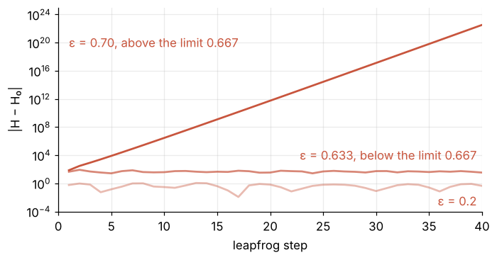
At ε = 0.2 the energy error stays below 1.13, at 0.633 it jumps to 84 within two steps and then swings below that without growing, and at 0.70 it grows to \(3 \times 10^{22}\). Leapfrog on an oscillator of period \(2\pi\sigma\) is stable only for \(\varepsilon < 2\sigma\), so the stiffest direction sets the limit, \(2\sigma_\min = 0.667\). Stable is not usable, though: from the second step on the error stays between 26 and 84, an acceptance below \(e^{-26}\), so practically every roll at 0.633 is rejected. The step that works sits well below the limit: ε = 0.2, under a third of it, accepts about 0.8 in the runs below. On the standard Gaussian of the question, where every σ is 1, the largest step that keeps the acceptance at 0.8 shrinks only slowly with the dimension:
Show code
def acceptance(q, p, eps, path=1.5):
    """Mean acceptance probability of leapfrog paths of length 1.5 on a standard Gaussian, one row per start."""
    q, p = q.copy(), p.copy()
    H0 = 0.5 * (q * q).sum(1) + 0.5 * (p * p).sum(1)
    for _ in range(math.ceil(path / eps)):
        p -= 0.5 * eps * q
        q += eps * p
        p -= 0.5 * eps * q
    dH = 0.5 * (q * q).sum(1) + 0.5 * (p * p).sum(1) - H0
    return np.minimum(1, np.exp(-dH)).mean()


print("      d   largest ε with acceptance ≥ 0.8   ε · d^(1/4)")
for d_std in [10, 100, 1_000, 10_000]:
    q, p = rng.standard_normal((500, d_std)), rng.standard_normal((500, d_std))   # exact draws: no chain needed
    lo, hi = 0.01, 1.5
    for _ in range(14):                                                           # bisection on ε
        mid = 0.5 * (lo + hi)
        lo, hi = (mid, hi) if acceptance(q, p, mid) >= 0.8 else (lo, mid)
    print(f"  {d_std:6,d}   {lo:31.3f}   {lo * d_std**0.25:11.2f}")
      d   largest ε with acceptance ≥ 0.8   ε · d^(1/4)
      10                             0.763          1.36
     100                             0.452          1.43
   1,000                             0.250          1.41
  10,000                             0.143          1.43
The product \(\varepsilon\, d^{1/4}\) stays near 1.4: from \(d\) = 10 to 10,000 the step shrinks by a factor of 5.3, where the random walk's \(2.38/\sqrt d\) shrinks by 32. The energy error is a sum of \(d\) per-direction errors, each with mean and variance of order \(\varepsilon^4\), so \(\varepsilon^4 d\) must stay fixed (Beskos et al. 2013). HMC's gradients per independent sample grow as \(d^{1/4}\), the random walk's evaluations as \(d\) (Neal 2011). On your own posterior, tune ε until the acceptance sits near 0.8, which the warmup of Stan and PyMC does by default (adapt_delta, target_accept).
Path length. At ε = 0.2 on the test bench, three ranges for \(L\), 60,000 gradients each:
Show code
print("  L drawn from   iterations   acceptance   τ / iterations   gradients per independent sample")
for L_range in [(2, 4), (6, 10), (12, 34)]:
    n = round(60_000 / np.mean(L_range))                     # 60,000 gradients for each row
    run = hmc(U_gauss, grad_gauss, chol @ rng.standard_normal(d), 0.2, L_range, n, rng)
    tau = integrated_time(run["chain"][:, None, 49:50], quiet=True)[0]
    print(f"  {L_range[0]:2d} to {L_range[1]:2d}   {n:12,d}   {run['acc']:10.2f}   {tau:14.2f}   "
          f"{run['work'][-1] / n * tau:32.0f}")
  L drawn from   iterations   acceptance   τ / iterations   gradients per independent sample
   2 to  4         20,000         0.80            47.60                                143
   6 to 10          7,500         0.84             7.10                                 57
  12 to 34          2,609         0.83             1.03                                 24
A short roll is a random walk with momentum: 143 gradients per independent sample of \(q_{50}\) at 2 to 4 steps, 24 at 12 to 34. The path \(\varepsilon L\) should be about a quarter period of the softest oscillator, \(\tfrac\pi2\sigma_\max = 4.7\), the swing from the center to the far edge; 12 to 34 steps of 0.2 cover 2.4 to 6.8. \(L\) is drawn at random because a fixed \(L\) can last exactly one period of some direction, which then never moves. On your own posterior, measure the gradients per independent sample in a short pilot run.
Divergences. On the banana the narrow direction narrows toward the tips, so a step that is stable in the bend is unstable up the arms. Stan stops a roll whose energy error passes 1,000 and counts it as divergent, and so does the code here:
Show code
def two_sigma_min(x):
    """2σ along the narrowest direction of the banana, on its ridge y = x² − 1."""
    hessian = np.array([[1 + 4 * x**2 / B**2, -2 * x / B**2], [-2 * x / B**2, 1 / B**2]])
    return 2 / math.sqrt(np.linalg.eigvalsh(hessian).max())


print("leapfrog stability limit 2σ_min across the ridge: "
      + ", ".join(f"{two_sigma_min(x):.2f} at x = {x}" for x in [0, 1, 2, 3]))
truth = math.erfc(2 / math.sqrt(2))                            # P(|x| > 2) for a standard normal x
print(f"\n   ε   acceptance   divergent of 10,000   share of samples with |x| > 2 (truth {truth:.4f})")
for eps in [0.08, 0.2]:
    with np.errstate(all="ignore"):                            # a divergent roll overflows before it is stopped
        run = hmc(U_banana, grad_banana, start, eps, (25, 25), 10_000, rng)
    tips = np.mean(np.abs(run["chain"][:, 0]) > 2)
    print(f"{eps:5.2f}   {run['acc']:10.3f}   {run['divergent'].sum():19,d}   {tips:15.4f}")
leapfrog stability limit 2σ_min across the ridge: 0.80 at x = 0, 0.35 at x = 1, 0.19 at x = 2, 0.13 at x = 3

   ε   acceptance   divergent of 10,000   share of samples with |x| > 2 (truth 0.0455)
 0.08        0.988                     0            0.0431
 0.20        0.783                   712            0.0117
The curvature across the ridge, the largest eigenvalue of the Hessian of \(U\), plays the spring constant \(1/\sigma^2\), so the stability limit falls from 0.80 at x = 0 to 0.19 at x = 2. At ε = 0.2, 712 of 10,000 rolls diverge, and the share of samples with \(|x| > 2\) is 0.0117 against the true 0.0455: three quarters of the tips are missing, while the acceptance, 0.783, looks healthy. At ε = 0.08 nothing diverges and the share is 0.0431. A divergence means that part of the posterior is not being visited. The fix is a smaller step or a reparametrization: sample \(z = (y - x^2 + 1)/0.4\), a round standard normal, and compute \(y\) from it.
See it in code
The cell runs both samplers on the test bench from the same exact draw of the target, so there is no burn-in: the random walk for 1,000,000 proposals at s = 0.112, keeping every tenth state, and HMC for 3,000 iterations at ε = 0.2 with \(L\) from 12 to 34. τ comes from integrated_time in emcee.autocorr, the estimator behind emcee's get_autocorr_time, converted to units of work:
Show code
q0 = chol @ rng.standard_normal(d)                 # an exact draw of the target: no burn-in
N_RW, THIN, N_HMC = 1_000_000, 10, 3_000
rw, rw_acc = rwm(lambda q: -U_gauss(q), q0, s_rw, N_RW, rng, thin=THIN)
hm = hmc(U_gauss, grad_gauss, q0, 0.2, (12, 34), N_HMC, rng)

# τ in units of work: density evaluations for the walk, gradients for HMC
tau_rw = THIN * integrated_time(rw[:, None, :], quiet=True)
tau_hmc = integrated_time(hm["chain"][:, None, :], quiet=True) * hm["work"][-1] / N_HMC
ess_rw, ess_hmc = 1e4 / tau_rw, 1e4 / tau_hmc
print(f"acceptance          random walk {rw_acc:.3f} (theory 0.234)   HMC {hm['acc']:.2f}")
print(f"run length / τ      random walk {N_RW / tau_rw.max():.0f}   HMC {hm['work'][-1] / tau_hmc.max():.0f}   (worst coordinate)")
print(f"τ of q₅₀ in work    random walk {tau_rw[49]:,.0f}   HMC {tau_hmc[49]:.1f}")
print(f"ESS per 10,000      random walk {ess_rw[49]:.2f}   HMC {ess_hmc[49]:.0f}   ratio {ess_hmc[49] / ess_rw[49]:.0f}")
print(f"worst coordinate    random walk {ess_rw.min():.2f}   HMC {ess_hmc.min():.0f}   ratio {ess_hmc.min() / ess_rw.min():.0f}")

# The check: along the principal directions the target is 100 independent unit Gaussians,
# so each sample mean times sqrt(ESS) should be one standard normal draw.
lam, V = np.linalg.eigh(Sigma)
for name, chain, n, scale in [("random walk", rw, N_RW, THIN), ("HMC", hm["chain"], N_HMC, 1)]:
    y = chain @ V / np.sqrt(lam)
    ess = n / (scale * integrated_time(y[:, None, :], quiet=True))
    z = y.mean(axis=0) * np.sqrt(ess)
    print(f"rms of mean × √ESS  {name:11s} {np.sqrt(np.mean(z**2)):.2f}")

fig, axes = plt.subplots(2, 1, figsize=(7, 4.4), sharex=True, sharey=True)
work_rw = THIN * np.arange(1, len(rw) + 1)
axes[0].plot(work_rw[work_rw <= 30_000], rw[work_rw <= 30_000, 49], color=SECOND, lw=1)
shown = hm["work"] <= 30_000
axes[1].step(hm["work"][shown], hm["chain"][shown, 49], where="post", color=ACCENT, lw=1)
for ax, name, ess in [(axes[0], "random walk", ess_rw[49]), (axes[1], "HMC", ess_hmc[49])]:
    ax.text(0.99, 0.97, f"{name}: {ess:.3g} effective samples per 10,000", transform=ax.transAxes,
            ha="right", va="top", color=INK)
    ax.set(ylabel="q₅₀", ylim=(-3.6, 5), yticks=[-2, 0, 2])
axes[-1].set(xlabel="units of work (density or gradient evaluations)", xlim=(0, 30_000))
axes[-1].xaxis.set_major_formatter(lambda x, _: f"{x:,.0f}")
plt.show()
acceptance          random walk 0.239 (theory 0.234)   HMC 0.84
run length / τ      random walk 125   HMC 2162   (worst coordinate)
τ of q₅₀ in work    random walk 4,362   HMC 25.9
ESS per 10,000      random walk 2.29   HMC 386   ratio 168
worst coordinate    random walk 1.25   HMC 312   ratio 249
rms of mean × √ESS  random walk 0.96
rms of mean × √ESS  HMC         1.00
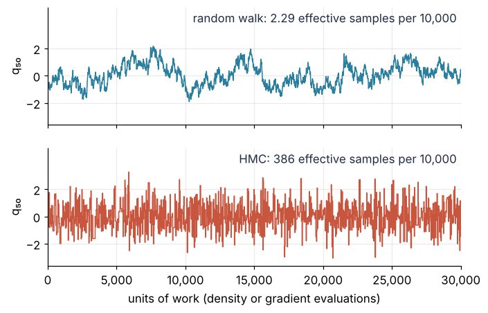
The random walk accepts 0.239 of its proposals, on the 0.234 its theory predicts, and both runs last more than 100 τ of their slowest coordinate. For \(q_{50}\), HMC gets 386 effective samples per 10,000 gradients and the random walk 2.29 per 10,000 density evaluations, a ratio of 168; for the slowest coordinate of each the ratio is 249. Whether those effective sample sizes are honest can be checked. Along the principal directions the target is 100 independent unit Gaussians, so each sample mean has the error \(1/\sqrt{\text{ESS}}\), the \(\sigma/\sqrt N\) of independent draws with ESS in place of \(N\). Each mean times \(\sqrt{\text{ESS}}\) should then be one draw from a standard normal, and the rms of the 100 should be near 1. It is 0.96 for the random walk and 1.00 for HMC. The random walk ran at the step its theory recommends, so the gap is information per unit of work, not an artifact of the estimator. Its size is less certain: other seeds put the ratio for \(q_{50}\) anywhere from 140 to 410, because the τ of so slow a walk is hard to pin down.
Where it shows up
The 100-dimensional Gaussian stands in for any posterior with many parameters and a log density that can be differentiated, and that describes most models fitted today.
- Lattice QCD (physics). HMC was invented there, as hybrid Monte Carlo, by Duane, Kennedy, Pendleton, and Roweth (Phys. Lett. B 195, 216, 1987), to sample gauge fields with millions of variables, where the fermion determinant makes updating one site at a time hopeless. It is still the standard algorithm for simulations with dynamical quarks.
- Stan and PyMC (statistics). Both sample with NUTS, HMC with the path length chosen per roll and with a step size and a mass matrix tuned during warmup. PyMC's
pm.sample()runs it by default for continuous parameters, and both report the divergences of every run. - Epidemiology and ecology (biology). The 2020 model of COVID-19 transmission across eleven European countries (Flaxman et al., Nature 2020) was fitted with Stan. Hierarchical models of populations and species with hundreds of parameters are fitted the same way.
- Pharmacokinetics (biology). Dose-response models whose concentrations obey ODEs are fitted with Stan's ODE solvers and with Torsten, a library of pharmacometric functions built on Stan. The gradient of the log density then runs through the ODE solver itself.
- Cosmology (physics). BORG reconstructs the initial density field of the local universe from galaxy surveys by HMC over millions of voxels (Jasche and Wandelt 2013). With τ growing in proportion to \(d\), the random walk's 338 proposals per independent draw at \(d\) = 100 would become millions.
- Bayesian neural networks (mathematics). Neal sampled the weights of neural networks with HMC in Bayesian Learning for Neural Networks (1996), the work that brought the method from physics into statistics. HMC on network weights is still the reference against which cheaper approximations are judged.
Wherever the log density has a gradient, it can be turned into a force, and a sampler that follows the force moves as far as it integrates accurately, not as far as it dares to guess.
Further reading
- R. M. Neal, "MCMC using Hamiltonian dynamics", in Handbook of Markov Chain Monte Carlo (Chapman and Hall/CRC, 2011), arXiv:1206.1901, for the algorithm and its proofs.
- M. Betancourt, "A conceptual introduction to Hamiltonian Monte Carlo" (2017), arXiv:1701.02434, for the geometry behind it and for divergences.
- M. D. Hoffman and A. Gelman, "The No-U-Turn sampler", J. Mach. Learn. Res. 15 (2014), for the sampler Stan and PyMC run.
- G. O. Roberts and J. S. Rosenthal, "Optimal scaling for various Metropolis-Hastings algorithms", Statistical Science 16 (2001), for the 0.234 and the random walk's step.
- The Stan Reference Manual, its chapter on MCMC sampling, for warmup and divergent transitions.
- The
emcee.autocorrdocumentation, forintegrated_time. - Related on this site: MCMC with emcee: the half-life and background of a counting experiment, Autocorrelation: how many independent hours a year of wind power holds, Symplectic integrators: why leapfrog's energy error is bounded and RK4's drifts, Velocity Verlet: keep the Earth on its orbit for a thousand years, the same leapfrog under another name, and Monte Carlo integration: why the error falls as one over the square root of N.
- Download the notebook. It was executed with the library versions in the header.