Monte Carlo integration: why the error falls as one over the square root of N (Python)

The question

Throw points at random into the unit square and count the share that lands inside the quarter circle of radius 1 around one corner. The quarter circle covers π/4 of the square, so four times that share estimates π. That is Monte Carlo integration in its simplest form, an area found by random sampling instead of by a formula. Here is one run with a million points:

Show code

import math
import numpy as np
import matplotlib.pyplot as plt

plt.rcParams.update({
    "figure.figsize": (8, 3.6), "figure.dpi": 110,
    "axes.spines.top": False, "axes.spines.right": False,
    "axes.grid": True, "grid.alpha": 0.25,
    "font.size": 11, "lines.linewidth": 1.8,
})
INK, ACCENT, SECOND, MUTED = "#1f2a44", "#c8553d", "#2a7f9e", "#8a8f98"

P = np.pi / 4                               # chance that one point lands inside
SIGMA = 4 * np.sqrt(P * (1 - P))            # scatter of one score of 4 or 0
CHUNK = 10**6

rng = np.random.default_rng(1)
xy = rng.random((CHUNK, 2))
inside = (xy**2).sum(axis=1) <= 1
scores = 4.0 * inside
n_pts = np.arange(1, CHUNK + 1)
running = np.cumsum(scores) / n_pts
s_open = scores.std(ddof=1)
print(f"N = {CHUNK:>11,}   estimate = {running[-1]:.4f} ± {s_open / np.sqrt(CHUNK):.4f}")

# continue the same stream to 10^8 points, a million at a time
hits, total = inside.sum(), CHUNK
for _ in range(99):
    hits += ((rng.random((CHUNK, 2))**2).sum(axis=1) <= 1).sum()
    total += CHUNK
p_hat = hits / total
print(f"N = {total:>11,}   estimate = {4 * p_hat:.5f} ± {4 * np.sqrt(p_hat * (1 - p_hat) / (total - 1)):.5f}")

fig, (ax1, ax2) = plt.subplots(1, 2, width_ratios=[1, 1.6], layout="constrained")
first = slice(0, 1000)
ax1.plot(*xy[first][inside[first]].T, "o", ms=2.5, color=ACCENT)
ax1.plot(*xy[first][~inside[first]].T, "o", ms=2.5, color=MUTED)
arc = np.linspace(0, np.pi / 2, 200)
ax1.plot(np.cos(arc), np.sin(arc), color=INK)
ax1.set(xlim=(0, 1), ylim=(0, 1), aspect="equal", xlabel="x", ylabel="y", xticks=[0, 1], yticks=[0, 1])
idx = np.unique(np.geomspace(10, CHUNK, 300).astype(int)) - 1
ax2.plot(n_pts[idx], running[idx], color=ACCENT)
ax2.axhline(np.pi, color=INK, lw=1)
ax2.text(CHUNK, np.pi - 0.03, "π", color=INK, ha="right", va="top")
ax2.text(CHUNK, np.pi + 0.03, f"{running[-1]:.4f}", ha="right", va="bottom", color=ACCENT)
ax2.set(xscale="log", xlim=(10, CHUNK), ylim=(2.9, 3.7), xlabel="N", ylabel="estimate of π")
plt.show()

N =   1,000,000   estimate = 3.1432 ± 0.0016
N = 100,000,000   estimate = 3.14154 ± 0.00016

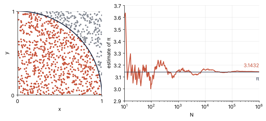
Left: 1,000 random points in the unit square, those inside the quarter circle highlighted. Right: the estimate of π against the number of points N on a log axis, wandering at first and settling near 3.14 by a million points.

The first thousand points already sketch the arc. Between 10 and 100 points the estimate swings by up to 0.5, between 100 and 1,000 by about 0.1, and after a million it reads 3.1432 ± 0.0016, three correct digits. Continuing the same random stream to 10⁸ points gives 3.14154 ± 0.00016: one more digit for a hundred times the points. I picked seed 1 because it is a typical run: π lies 1.0 and 0.3 error bars from its two estimates, an error bar being the ± that the next section derives. That section also shows a hundred other runs, so nothing here rests on the pick.

Two things are obvious. The estimate converges, and it converges slowly.

Less obvious: why exactly a factor of ten in the error for a factor of a hundred in N, and where the ± comes from, when a real calculation does not know the answer it is estimating. And there is an obvious alternative. Lay the same million points on a regular grid instead of at random: a grid leaves no gaps and has no clusters, so it sounds at least as good. Whether it is depends on the dimension, more strongly than you would guess.

The idea: the fraction is an average

Look at a single point. It lands inside with probability p = π/4 and scores 4, or outside and scores 0. The estimate after N points is the mean of N such scores, nothing more. So it scatters like any mean of N independent values: the scatter of one score, σ, divided by √N. A hundred times the points divides the error by ten.

σ follows from the two outcomes. A score that is 4 with probability p and 0 otherwise has the mean 4p = π and the standard deviation σ = 4√(p(1 − p)), which is 1.642 for p = π/4. Single scores are as scattered as they come, every one of them off from π by 0.86 or by 3.14. Only their mean is precise.

To check the prediction, run the experiment a hundred times, each run to N = 10⁵ with a generator seeded once (seeding is the subject of Random numbers with numpy.random), and draw the bands π ± σ/√N and π ± 2σ/√N around the truth:

Show code

N_RUN, RUNS = 10**5, 100
rng = np.random.default_rng(2026)
n_run = np.arange(1, N_RUN + 1)
runs = np.array([np.cumsum(4.0 * ((rng.random((N_RUN, 2))**2).sum(axis=1) <= 1)) / n_run
                 for _ in range(RUNS)])

half = SIGMA / np.sqrt(N_RUN)
miss = np.abs(runs[:, -1] - np.pi)
in1, in2 = (miss < half).sum(), (miss < 2 * half).sum()
print(f"inside π ± σ/√N at N = 10^5:  {in1:3d} of {RUNS}")
print(f"inside π ± 2σ/√N at N = 10^5: {in2:3d} of {RUNS}")
print(f"opening run: s = {s_open:.3f}   true σ = {SIGMA:.3f}")

fig, ax = plt.subplots(figsize=(7, 3.6))
grid_n = np.geomspace(100, N_RUN, 300)
idx = np.unique(np.geomspace(100, N_RUN, 200).astype(int)) - 1
for r in runs:
    ax.plot(n_run[idx], r[idx], color=ACCENT, lw=0.6, alpha=0.3)
for k, alpha in [(2, 0.15), (1, 0.30)]:
    lo_k, hi_k = np.pi - k * SIGMA / np.sqrt(grid_n), np.pi + k * SIGMA / np.sqrt(grid_n)
    ax.fill_between(grid_n, lo_k, hi_k, color=MUTED, alpha=alpha, lw=0, zorder=0)
    ax.plot(grid_n, lo_k, grid_n, hi_k, color=MUTED, lw=1, zorder=3)     # band edges above the runs
ax.axhline(np.pi, color=INK, lw=1, zorder=3)
ax.text(N_RUN, 3.52, f"at N = 10⁵: {in1} of {RUNS} inside ±σ/√N,\n{in2} inside ±2σ/√N",
        color=INK, ha="right", va="top")
ax.set(xscale="log", xlim=(100, N_RUN), ylim=(2.6, 3.62), xlabel="N", ylabel="estimate of π")
plt.show()

inside π ± σ/√N at N = 10^5:   69 of 100
inside π ± 2σ/√N at N = 10^5:  98 of 100
opening run: s = 1.641   true σ = 1.642

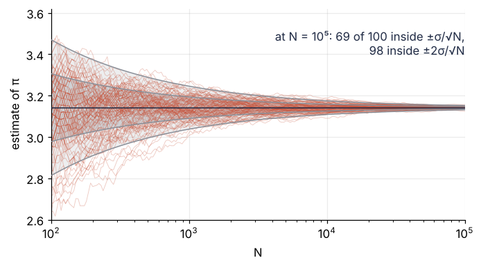
One hundred independent estimates of π against N on a log axis, inside bands of one and two standard errors, σ/√N, that narrow as N grows; about two thirds end inside the inner band.

At N = 10⁵, 69 of the 100 runs end inside the inner band and 98 inside the outer one, against the 68 and 95 that a normal distribution of means predicts. The bands narrow by √10 = 3.2 per decade of N, and the runs narrow with them.

The bands are drawn around the true π, with the true σ, only to show the scatter. A real run knows neither. It uses the sample standard deviation s of its own scores in place of σ, and for the opening run that is 1.641 against the true 1.642. The ± of the opening, 0.0016 at a million points, is s/√N computed exactly that way, from the same million scores that gave the estimate.

Here is the opening run again, as it happens. The points fill the square, and the estimate on the right falls into the narrowing bands and stays there:

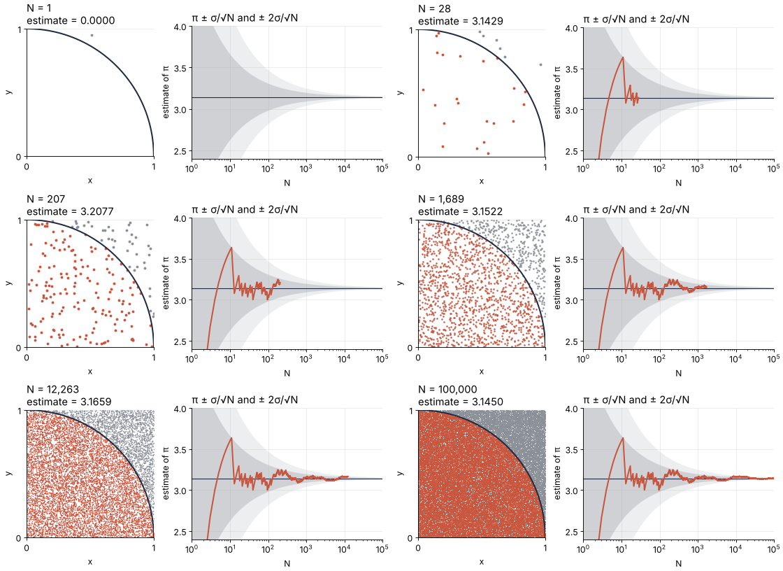
Left: random points fall into the unit square, those inside the quarter circle in red, with N and the current estimate of π above. Right: the running estimate against N on a log axis, settling inside bands of one and two σ/√N around π as N grows to 100,000.

How I built this: each frame shows the first N points of the opening run and the running estimate up to N, drawn with Matplotlib's FuncAnimation, the technique of Matplotlib animation with FuncAnimation; the source is animations/points-rain/scene.py.

A grid of the same points: better in one dimension, worse in ten

Now the alternative. In one dimension the quarter circle is an ordinary integral, π = 4∫₀¹√(1 − x²) dx, and the standard way to compute it is a grid. The midpoint rule cuts [0, 1] into N cells of width h = 1/N and adds the integrand at each cell's center, times h. How fast a rule improves is its order p, a different p from the probability of the darts: its error is proportional to hᵖ, a straight line of slope −p on a log-log plot against N. Monte Carlo averages the same integrand at N random points.

In ten dimensions the question is the volume of the unit ball, all points with x₁² + … + x₁₀² ≤ 1, inside the cube [−1, 1]¹⁰. Its volume is 2¹⁰ times the share of points inside, whether the points are random or on a grid of k points per axis:

Show code

# one dimension: pi as the integral of 4 sqrt(1 - x^2) over [0, 1]
f1 = lambda x: 4 * np.sqrt(1 - x**2)
rng = np.random.default_rng(2026)
Ns = 10 ** np.arange(1, 7)
err_grid = np.array([abs(f1((np.arange(N) + 0.5) / N).mean() - np.pi) for N in Ns])
fx = [f1(rng.random(N)) for N in Ns]
err_mc = np.array([abs(v.mean() - np.pi) for v in fx])
se_mc = np.array([v.std(ddof=1) / np.sqrt(v.size) for v in fx])
print(f"1D, N = 1,000: grid error {err_grid[2]:.1e}   Monte Carlo standard error {se_mc[2]:.3f}")

# ten dimensions: the unit ball inside [-1, 1]^10
D, V = 10, 2.0**10
EXACT = np.pi**5 / 120

def grid_volume(k, d=D):
    """Ball volume from a k^d midpoint grid, by counting sums of squares instead of building the grid."""
    sq = (2 * np.arange(k) + 1 - k) ** 2          # squared coordinates in units of 1/k^2, exact integers
    counts = np.ones(1, dtype=np.int64)
    for _ in range(d):
        counts = np.convolve(counts, np.bincount(sq))
    return V * counts[: k * k + 1].sum() / k**d

ks = np.arange(2, 7)
grid_vol = np.array([grid_volume(k) for k in ks])

checkpoints = np.unique(np.geomspace(1e3, 1e7, 9).astype(int))
rng = np.random.default_rng(2026)
hits, done, mc_vol, mc_err = 0, 0, [], []
for N in checkpoints:
    while done < N:
        m = min(CHUNK, N - done)
        hits += ((rng.uniform(-1, 1, (m, D))**2).sum(axis=1) <= 1).sum()
        done += m
    p_hat = hits / done
    mc_vol.append(V * p_hat)
    mc_err.append(V * np.sqrt(p_hat * (1 - p_hat) / (done - 1)))
for N, v, e in zip(checkpoints, mc_vol, mc_err):
    if N in (10**6, 10**7):
        print(f"10D, N = {N:>10,}: Monte Carlo {v:.3f} ± {e:.3f}   exact {EXACT:.4f}")
print("10D grid volumes, k = 2 to 6:", "  ".join(f"{v:.2f}" for v in grid_vol))

fig, (ax1, ax2) = plt.subplots(1, 2, layout="constrained")
ax1.loglog(Ns, err_mc, "o", ms=6, color=ACCENT)
ax1.loglog(Ns, err_grid, "o", ms=6, color=SECOND)
ax1.text(3e3, 0.3, "random points", color=ACCENT, ha="center", va="center")
ax1.text(12, 1e-6, "midpoint grid", color=SECOND, ha="left", va="center")
guides = {"−1/2": fx[-1].std(ddof=1) / np.sqrt(Ns), "−3/2": 0.05 * (Ns / 10.0) ** -1.5}   # predicted scatter, and a slope
for label, y in guides.items():
    ax1.loglog(Ns, y, color=MUTED, lw=1, ls="--")
    ax1.text(Ns[-1] * 1.8, y[-1], label, color=MUTED, va="center")
ax1.set(xlabel="N", ylabel="|error|", xlim=(5, 1.5e7), ylim=(1e-10, 2))
ax2.errorbar(checkpoints, mc_vol, yerr=mc_err, fmt="o", ms=4, capsize=2, lw=1, color=ACCENT)
ax2.plot(ks.astype(float) ** D, grid_vol, "s", ms=6, color=SECOND)
for k, Nk, v in zip(ks, ks.astype(float) ** D, grid_vol):
    side = dict(xytext=(8, 0), ha="left", va="center") if k == 2 else dict(xytext=(0, 7), ha="center")
    ax2.annotate(f"k = {k}", (Nk, v), textcoords="offset points", color=SECOND, **side)
ax2.axhline(EXACT, color=INK, lw=1)
ax2.text(1.8e8, EXACT - 0.12, f"exact {EXACT:.3f}", color=INK, ha="right", va="top")
ax2.set(xscale="log", xlabel="N", ylabel="volume of 10D ball", ylim=(-0.3, 5.2), xlim=(5e2, 2e8))
plt.show()

1D, N = 1,000: grid error 1.1e-05   Monte Carlo standard error 0.029
10D, N =  1,000,000: Monte Carlo 2.526 ± 0.051   exact 2.5502
10D, N = 10,000,000: Monte Carlo 2.545 ± 0.016   exact 2.5502
10D grid volumes, k = 2 to 6: 0.00  3.49  1.00  3.07  3.23

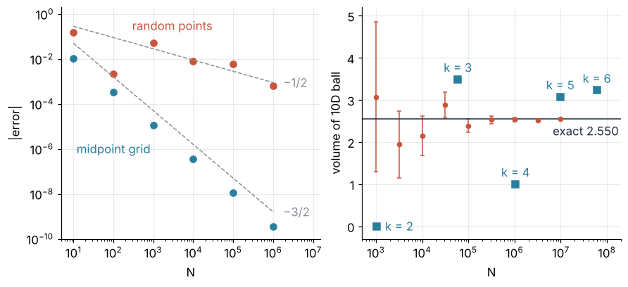
Left: error against N in one dimension, log-log; the midpoint grid falls with slope −3/2, random points with slope −1/2. Right: volume of the ten-dimensional ball against N; grid values jump between 0 and 3.5, Monte Carlo settles on the exact 2.55.

In one dimension the grid wins by a mile. Its error falls by a factor of 31 per decade of N, a slope of −3/2, and at N = 1,000 it is 1.1 × 10⁻⁵, against a Monte Carlo standard error of 0.029. The midpoint rule normally has order 2, but near x = 1 the integrand behaves like √(1 − x), whose slope is infinite there, and the last cell alone contributes an error of order h^(3/2). Nothing offsets it: the curve bends downward everywhere, so the midpoint value overestimates every cell. The errors of single Monte Carlo runs scatter about the line the previous section predicts, the scatter of 4√(1 − x²) itself over √N, a new σ and not the 1.642 of the darts: a factor of 3.2 per decade, a slope of −1/2.

In ten dimensions the order is reversed. Grids of k = 2 to 6 points per axis, 1,024 to 60 million points, give 0, 3.49, 1.00, 3.07, and 3.23 for a ball whose volume is 2.550, while Monte Carlo reaches 2.526 ± 0.051 at 10⁶ points and 2.545 ± 0.016 at 10⁷. The grid values are not noise but accidents of geometry. With k = 4 each coordinate is ±0.25 or ±0.75, and a single coordinate at ±0.75 adds 0.5625 to the sum of squares, the other nine add at least 0.0625 each, and the total of at least 1.125 is past 1. Only the 2¹⁰ points with every coordinate at ±0.25 count, and the grid reports 2¹⁰ × 2¹⁰/4¹⁰ = 1.000 whatever the ball's real shape. With k = 2 every coordinate is ±0.5, the sum of squares is 2.5, and no point is inside at all. Each k makes a different accident, which is why the values jump instead of converging.

What makes the grid's error depend on the dimension, and Monte Carlo's not?

Formalization

The darts are one case of a general statement. For a point X drawn uniformly from a region of volume V, the integral of f over the region is V times the expected value of f(X), and the mean over N independent points estimates it:

\[\int f(\mathbf{x})\,d\mathbf{x} = V\,\mathrm{E}[f(X)] \approx \frac{V}{N}\sum_{i=1}^{N} f(X_i).\]

For π the region is the unit square, V = 1, and f is four times the indicator of the disk, the function that is 1 inside and 0 outside.

The error follows from two rules about variances. Variances of independent values add, so the sum of the N values f(Xᵢ) has the variance \(N\sigma_f^2\), with \(\sigma_f\) the standard deviation of a single value; dividing the sum by N divides the variance by N². What remains is the standard error

\[\mathrm{SE} = \frac{V\,\sigma_f}{\sqrt{N}}.\]

The standard error of the mean derives the same 1/√N with pictures. Three consequences follow.

One more digit costs a hundred times the points. The opening run went from 0.0016 at 10⁶ points to 0.00016 at 10⁸. Nothing in \(V\sigma_f/\sqrt{N}\) mentions the dimension: the exponent is −1/2 on a line and in a thousand dimensions. The constant \(\sigma_f\) does depend on the integrand. Only 0.25 % of the ten-dimensional cube is ball, so nearly every point scores zero, and the error bar at 10⁶ points is 2 % of the result against 0.05 % for π.

The error bar comes from the same samples, for any f. \(\sigma_f\) is as unknown as the integral. The sample standard deviation \(s_f\) of the N values f(Xᵢ) replaces it, and the result is reported as \(V\,\overline{f} \pm V s_f/\sqrt{N}\), with \(\overline{f}\) their mean. The opening run did exactly this with its scores of 4 and 0, and the 69 of 100 runs inside the one-standard-error band are the check that the error bar is honest.

A grid's error depends on the dimension. N grid points in d dimensions give k = N^(1/d) points per axis and a spacing h proportional to 1/k, so a rule of order p has an error of order hᵖ = N^(−p/d). Monte Carlo's N^(−1/2) falls faster once p/d < 1/2, that is in more than 2p dimensions. The midpoint rule has p = 2, and it keeps that order on the ball despite the jump of the indicator at the surface. The surface cuts many cells, each counted fully or not at all, some too much and some too little, and over the curved surface these errors cancel on average. That is what fails on a line: for √(1 − x²) every cell erred upward, and a single jump cuts one cell, which can be off by half its width, an error of order h. The remainder depends on how the grid lines up with the surface, so its sign changes from k to k, +1.97 % at 15 points per axis and −3.85 % at 16, but its size shrinks as h²: from 16 to 32 and 64 points it falls fourfold per doubling, to −0.96 % and −0.24 %. So the crossover is at four dimensions, and in ten the grid's error falls as N^(−1/5) against Monte Carlo's N^(−1/2). An affordable grid, 4 to 6 points per axis, is too coarse to see the ball at all, and that is where the accidents come from:

Show code

print(" k                          N    grid volume      error")
for k in [2, 3, 4, 5, 6, 7, 15, 16, 32, 64]:
    v = grid_volume(k)
    print(f"{k:2d} {k**D:>26,}    {v:11.3f}    {100 * (v - EXACT) / EXACT:+7.2f} %")

 k                          N    grid volume      error
 2                      1,024          0.000    -100.00 %
 3                     59,049          3.486     +36.68 %
 4                  1,048,576          1.000     -60.79 %
 5                  9,765,625          3.071     +20.41 %
 6                 60,466,176          3.226     +26.48 %
 7                282,475,249          2.775      +8.83 %
15            576,650,390,625          2.600      +1.97 %
16          1,099,511,627,776          2.452      -3.85 %
32      1,125,899,906,842,624          2.526      -0.96 %
64  1,152,921,504,606,846,976          2.544      -0.24 %

Seven points per axis cost 2.8 × 10⁸ evaluations and still miss by 9 %, more than four times the 2 % error bar that Monte Carlo had at 10⁶ points. The grid first gets inside that 2 % at 15 points per axis, with 5.8 × 10¹¹ evaluations, half a million times what Monte Carlo spent.

Monte Carlo pays for its rate with one condition: the samples must be independent. When each sample is drawn from the one before, which is what a Markov chain does, N correlated samples carry the information of fewer independent ones, the effective N, and the √N in the error bar must be that number. If the correlation between samples i steps apart falls as 0.9ⁱ, the effective N is N(1 − 0.9)/(1 + 0.9), one in nineteen.

See it in code

The whole method fits in one function. It draws N points uniformly in a box, evaluates the integrand at all of them, and returns the box volume times the mean and times the standard error. Here it is applied in [−1, 1]¹⁰ to the ball's indicator and to the smooth exp(−|x|²). The exact values are π^(d/2)/Γ(d/2 + 1) for the ball, where Γ extends the factorial so that Γ(6) = 5! = 120, and (√π erf 1)¹⁰ for the Gaussian, a product of ten one-dimensional integrals:

Show code

def mc_integrate(f, lo, hi, n, rng):
    """Integral of f over the box [lo, hi] from n uniform points, and its standard error."""
    lo, hi = np.asarray(lo, float), np.asarray(hi, float)
    volume = np.prod(hi - lo)
    fx = f(rng.uniform(lo, hi, (n, lo.size)))       # one row per point
    return volume * fx.mean(), volume * fx.std(ddof=1) / np.sqrt(n)

rng = np.random.default_rng(2026)
d, n = 10, 4**10
lo, hi = -np.ones(d), np.ones(d)
ball = lambda x: ((x**2).sum(axis=1) <= 1).astype(float)
gauss = lambda x: np.exp(-(x**2).sum(axis=1))

ball_exact = np.pi ** (d / 2) / math.gamma(d / 2 + 1)
gauss_exact = (math.sqrt(math.pi) * math.erf(1)) ** d
ball_mc, ball_se = mc_integrate(ball, lo, hi, n, rng)
gauss_mc, gauss_se = mc_integrate(gauss, lo, hi, n, rng)
print(f"ball,     Monte Carlo:     {ball_mc:7.3f} ± {ball_se:.3f}   exact {ball_exact:7.3f}")
print(f"ball,     4-per-axis grid: {grid_volume(4):7.3f}           exact {ball_exact:7.3f}")
print(f"Gaussian, Monte Carlo:     {gauss_mc:7.3f} ± {gauss_se:.3f}   exact {gauss_exact:7.3f}")
print(f"distance from exact in error bars: ball {(ball_mc - ball_exact) / ball_se:+.2f}, "
      f"Gaussian {(gauss_mc - gauss_exact) / gauss_se:+.2f}")

ball,     Monte Carlo:       2.518 ± 0.050   exact   2.550
ball,     4-per-axis grid:   1.000           exact   2.550
Gaussian, Monte Carlo:      55.291 ± 0.054   exact  55.269
distance from exact in error bars: ball -0.66, Gaussian +0.40

Both exact values lie within the error bar: the ball's estimate is 0.66 error bars below 2.550, the Gaussian's 0.40 above 55.269. The grid of the same 4¹⁰ points is off by 61 %, and nothing in its output says so. The Gaussian gets an error bar of 0.1 % at the same N where the ball gets 2 %, because its values scatter far less about their mean than a 0 or 1 does: the same rate, a smaller \(\sigma_f\). For your own integral, change the lambda and the box. Of the answers printed, only the error bars tell you how far to trust them.

Where it shows up

Engineering. Shielding around a reactor is designed with codes such as MCNP and OpenMC, which follow individual neutrons through scattering and absorption in the wall. The fraction that gets through is a hit count like the darts, and every tally comes with its statistical error, in MCNP as a relative error.
Physics. Radiotherapy dose is computed by photon and electron transport with EGSnrc or Geant4, one particle history at a time. The dose in each voxel of the patient is an average over the histories that deposit energy there, and it carries its own error bar.
Chemistry. The average energy of a liquid is an integral over the 3N coordinates of its molecules, weighted by the Boltzmann factor exp(−E/kT), which is nearly zero almost everywhere, so uniform points like the darts would almost all land where nothing counts. The Metropolis algorithm samples in proportion to that factor instead, each step from the one before, so the effective N is smaller than the number of steps.
Geology. The event-based calculator of the OpenQuake engine simulates many synthetic earthquake catalogs for a region and counts the events whose shaking at a site exceeds a given level. That count per catalog is a Monte Carlo mean like the darts, and a Poisson model turns it into the probability of exceedance.
Biology. MrBayes and BEAST report the posterior probability of a branch in a phylogenetic tree as the share of Markov chain samples that contain it, the same mean of samples with an effective sample size in place of N. MCMC with emcee does the same for a counting experiment in Python.

In every case the error is the integrand's scatter divided by the square root of the number of independent samples, whatever the dimension.

The question

The idea: the fraction is an average

A grid of the same points: better in one dimension, worse in ten

Formalization

See it in code

Where it shows up

Further reading