Velocity Verlet: keep the Earth on its orbit for a thousand years (Python)

The problem: does the Earth stay on its orbit for a thousand years?

Put the Earth on its real orbit, eccentricity 0.0167, around a fixed Sun, and give it to solve_ivp with the default settings for a thousand years. It never gets there. After one year the Earth has lost 5 % of its orbital energy, after ten years its semimajor axis is down to 0.36 AU, and at year 12.8 the solver gives up with "Required step size is less than spacing between numbers". The Earth has fallen into the Sun.

Velocity Verlet does the same job in four lines of code per step with one force evaluation, and its energy error stays bounded instead of growing. That is why it is the standard integrator of molecular dynamics, where a simulation of a protein or a liquid lasts millions of steps, and inside many long orbit integrations. Written by hand in NumPy, it is about ten lines.

The check throughout is the energy per unit mass,

\[E = \tfrac12 v^2 - \frac{GM}{r},\]

with \(v\) the speed, \(r\) the distance from the Sun, and \(GM\) the Sun's gravitational parameter. On an orbit of semimajor axis \(a\) it stays at \(-GM/(2a)\) forever, so any change in it is the integrator's doing.

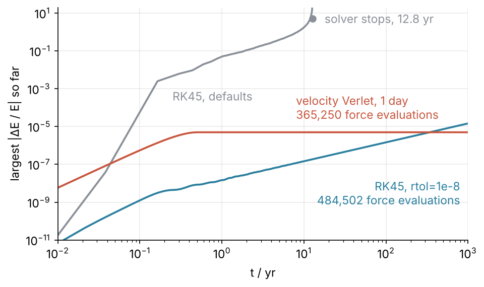
Largest relative energy error so far against time in years, both axes logarithmic, over 1000 years. RK45 at default tolerances passes 100 % and stops at 12.8 years; RK45 at rtol 1e-8 grows in proportion to time; velocity Verlet stays flat at 5e-6.

The figure shows the largest relative energy error so far for three runs. RK45 at default tolerances climbs past 100 % and ends where the solver stopped. RK45 at rtol=1e-8 is far better at first but grows in proportion to time. Velocity Verlet at one step per day stays at 5 × 10⁻⁶ from the first year to the thousandth and overtakes the tight RK45 near year 340. Step 6 draws it.

Setup

import numpy as np
import matplotlib.pyplot as plt
from scipy.integrate import solve_ivp

GM = 4 * np.pi**2    # AU^3/yr^2; with masses in solar masses this is G
e = 0.0167           # eccentricity of the Earth's orbit
DAY = 1 / 365.25     # yr

plt.rcParams.update({
    "figure.figsize": (7, 3.6), "figure.dpi": 110,
    "axes.spines.top": False, "axes.spines.right": False,
    "axes.grid": True, "grid.alpha": 0.25,
    "font.size": 11, "lines.linewidth": 1.8,
})
INK, ACCENT, SECOND, MUTED = "#1f2a44", "#c8553d", "#2a7f9e", "#8a8f98"

print(f"target energy -GM/(2a) for a = 1 AU: {-GM / 2:.4f} AU²/yr²")

target energy -GM/(2a) for a = 1 AU: -19.7392 AU²/yr²

Step 1: Write the Kepler problem in AU, years, and solar masses

Kepler's third law says that an orbit of semimajor axis \(a\) takes \(T = 2\pi\sqrt{a^3/GM}\). Measure lengths in astronomical units and time in years, and \(T = 1\) yr at \(a = 1\) AU forces \(GM = 4\pi^2\). No large exponents, and the exact orbit returns to its start after exactly one year. The Sun is held fixed and the Earth's mass, 3 × 10⁻⁶ solar masses, is neglected; with \(G(M + m)\) in place of \(GM\) the two-body problem in relative coordinates is exactly this one. With masses counted in solar masses, the Sun's mass is 1 and \(GM\) is the gravitational constant \(G\) itself, which Step 5 multiplies by the planets' masses.

The energy also fixes the size of the orbit, \(a = -GM/(2E)\). An energy error is therefore an orbit of the wrong size. The Earth starts at perihelion, at distance \(1 - e\), moving perpendicular to the Sun at the speed the vis-viva law \(v^2 = GM(2/r - 1/a)\) gives there. The cell also prints \(\tau = r/v\) at perihelion, the time the Earth needs to cover its own distance from the Sun; Step 4 picks the time step from it.

def accel(r):
    """Acceleration toward the fixed Sun; r has x, y on its last axis."""
    return -GM * r / np.linalg.norm(r, axis=-1, keepdims=True) ** 3

def energy(r, v):
    return 0.5 * np.sum(v**2, axis=-1) - GM / np.linalg.norm(r, axis=-1)

r0 = np.array([1 - e, 0.0])                              # AU, perihelion
v0 = np.array([0.0, np.sqrt(GM * (1 + e) / (1 - e))])    # AU/yr
E0 = energy(r0, v0)
print(f"E0 = {E0:.4f} AU²/yr²   a = -GM/(2 E0) = {-GM / (2 * E0):.4f} AU")
print(f"tau = r/v at perihelion: {np.linalg.norm(r0) / np.linalg.norm(v0) * 365.25:.0f} days")

E0 = -19.7392 AU²/yr²   a = -GM/(2 E0) = 1.0000 AU
tau = r/v at perihelion: 56 days

Both functions work on a single state or on a whole time series at once, because they reduce over the last axis only.

Step 2: Run solve_ivp for a thousand years and watch the energy

solve_ivp wants a first-order system, so the state is \((x, y, v_x, v_y)\) and the right-hand side returns the velocity and the acceleration. Tolerances, nfev, and the energy check are the subject of solve_ivp from the ground up. First the defaults:

def rhs(t, y):
    return np.concatenate([y[2:], accel(y[:2])])

y0 = np.concatenate([r0, v0])
sol = solve_ivp(rhs, (0, 1000), y0, dense_output=True)
print(f"status {sol.status}: {sol.message}")
print(f"stopped at t = {sol.t[-1]:.1f} yr")
for t in [1, 5, 10]:
    E = energy(sol.sol(t)[:2], sol.sol(t)[2:])
    print(f"t = {t:2d} yr   energy error {abs(E / E0 - 1):6.1%}   a = {-GM / (2 * E):.2f} AU")

t_default = sol.t
err_default = np.abs(energy(sol.y[:2].T, sol.y[2:].T) / E0 - 1)

status -1: Required step size is less than spacing between numbers.
stopped at t = 12.8 yr
t =  1 yr   energy error   4.9%   a = 0.95 AU
t =  5 yr   energy error  38.8%   a = 0.72 AU
t = 10 yr   energy error 174.3%   a = 0.36 AU

The energy falls by 5 % in the first year, and by Step 1's relation the orbit shrinks to 0.95 AU, then to 0.36 AU by year 10. At year 12.8 the Earth passes so close to the Sun that the step the solver needs is smaller than the spacing of floating-point numbers. Now with tight tolerances:

tight = solve_ivp(rhs, (0, 1000), y0, rtol=1e-8, atol=1e-11)
err_tight = np.abs(energy(tight.y[:2].T, tight.y[2:].T) / E0 - 1)
print(f"{len(tight.t) - 1} steps, nfev = {tight.nfev}")
for t in [1, 10, 100, 1000]:
    print(f"t = {t:4d} yr   largest energy error so far {err_tight[tight.t <= t].max():.2e}")

74502 steps, nfev = 484502
t =    1 yr   largest energy error so far 1.46e-08
t =   10 yr   largest energy error so far 1.46e-07
t =  100 yr   largest energy error so far 1.46e-06
t = 1000 yr   largest energy error so far 1.46e-05

It reaches the thousand years, and the error is small. But ten times the time gives ten times the error, decade after decade. Each step makes a tiny energy error with a sign, and the signs do not cancel. Run long enough and any such error becomes large.

Step 3: Write velocity Verlet: half a kick, a drift, half a kick

The position takes a Taylor step to second order, \(r \leftarrow r + v\,\Delta t + a\,\Delta t^2/2\), and the velocity advances by the average of the old and the new acceleration, \(v \leftarrow v + (a_\text{old} + a_\text{new})\,\Delta t/2\). Split that velocity update into its two halves and the same algebra reads

\[v \leftarrow v + \tfrac{\Delta t}{2}\,a(r), \qquad r \leftarrow r + \Delta t\, v, \qquad v \leftarrow v + \tfrac{\Delta t}{2}\,a(r):\]

a half kick, a drift, a half kick. The force of the last half kick is the force of the next step's first, so each step costs one force evaluation. (On a grid the same scheme is the leapfrog of the wave equation with leapfrog finite differences.)

def verlet(accel, r0, v0, dt, n):
    r = np.empty((n + 1, *r0.shape))
    v = np.empty_like(r)
    r[0], v[0] = r0, v0
    a = accel(r0)
    for k in range(n):
        v_half = v[k] + 0.5 * dt * a
        r[k + 1] = r[k] + dt * v_half
        a = accel(r[k + 1])                  # reused as the first half kick of the next step
        v[k + 1] = v_half + 0.5 * dt * a
    return r, v

dt = DAY
r, v = verlet(accel, r0, v0, dt, 365_250)
err_verlet = np.abs(energy(r, v) / E0 - 1)
t_verlet = dt * np.arange(len(r))
print(f"largest energy error in year 1:    {err_verlet[:366].max():.2e}")
print(f"largest energy error in year 1000: {err_verlet[-366:].max():.2e}")

largest energy error in year 1:    4.97e-06
largest energy error in year 1000: 4.97e-06

The same error in the last year as in the first. Over the first three years it looks like this:

first = t_verlet <= 3
fig, ax = plt.subplots(figsize=(7, 3.4))
ax.plot(t_verlet[first], err_verlet[first] * 1e6, color=ACCENT)
for year in range(3):
    ax.text(year + 0.5, 5.2, "aphelion", ha="center", color=MUTED)
for year in [1, 2]:
    ax.annotate("perihelion", xy=(year, 0.15), xytext=(year, 3.2), ha="center", color=MUTED,
                arrowprops=dict(arrowstyle="->", color=MUTED, lw=1))
ax.set(xlabel="t / yr", ylabel="|ΔE / E| / 10⁻⁶", xlim=(0, 3), ylim=(0, 6))
plt.show()

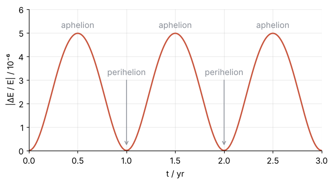
Relative energy error of velocity Verlet over the first three years at a step of one day. It rises from zero at perihelion to 5e-6 at aphelion and returns to zero, once per orbit, without growing.

Zero at perihelion, 5 × 10⁻⁶ at aphelion, once per orbit, and no trend.

Here is why. A kick changes only velocities, by an amount set by the positions; a drift changes only positions, by an amount set by the velocities. Each is a shear, and a shear keeps the area of any patch of starting states drawn with positions against velocities. A method built from such steps is called symplectic. A symplectic method conserves a nearby "shadow" energy almost exactly, up to an error so small that it shows only after a number of steps that grows exponentially with \(1/\Delta t\), and the shadow energy differs from the true energy by a term of order \(\Delta t^2\). So the true energy can only wobble around a fixed value. The geometry behind this deserves its own tutorial, which is planned.

Step 4: Check it against the exact orbit and choose the time step

A method of order \(p\) has an error proportional to \(\Delta t^p\): halving \(\Delta t\) divides the error by \(2^p\), and a factor 4 means \(p = 2\). The exact Earth is back at its start after one year, which gives a second check, the position error. One orbit at 48 to 768 steps:

steps = [48, 96, 192, 384, 768]
dE, dr = [], []
for n in steps:
    r1, v1 = verlet(accel, r0, v0, 1 / n, n)
    dE.append(np.abs(energy(r1, v1) / E0 - 1).max())
    dr.append(np.linalg.norm(r1[-1] - r0))       # the exact Earth is back at r0

print(" dt / day   energy error   ratio   position error / AU   ratio")
for k, n in enumerate(steps):
    ratio_E = f"{dE[k - 1] / dE[k]:5.2f}" if k else ""
    ratio_r = f"{dr[k - 1] / dr[k]:5.2f}" if k else ""
    print(f"{365.25 / n:8.3f}   {dE[k]:12.2e}   {ratio_E:>5s}   {dr[k]:19.2e}   {ratio_r:>5s}")

 dt / day   energy error   ratio   position error / AU   ratio
   7.609       3.55e-04                      3.69e-02        
   3.805       7.60e-05    4.67              9.25e-03    3.98
   1.902       1.82e-05    4.18              2.32e-03    4.00
   0.951       4.50e-06    4.05              5.79e-04    4.00
   0.476       1.12e-06    4.01              1.45e-04    4.00

Both errors fall by a factor of 4 per halving: velocity Verlet is second order.

The energy error is bounded. Is the position error? Compare the first and the last orbit of Step 3's run:

for name, orbit in [("first", slice(0, 366)), ("last", slice(-366, None))]:
    dist = np.linalg.norm(r[orbit], axis=1)
    r_peri = r[orbit][dist.argmin()]
    print(f"{name:5s} orbit: a = {(dist.max() + dist.min()) / 2:.5f} AU,"
          f" e = {(dist.max() - dist.min()) / (dist.max() + dist.min()):.5f},"
          f" perihelion at {np.degrees(np.arctan2(r_peri[1], r_peri[0])):6.1f}°")
print(f"distance from the exact Earth after 1000 yr: Verlet {np.linalg.norm(r[-1] - r0):.2f} AU,"
      f" tight RK45 {np.linalg.norm(tight.y[:2, -1] - r0):.2f} AU")

first orbit: a = 1.00008 AU, e = 0.01678, perihelion at    0.0°
last  orbit: a = 1.00008 AU, e = 0.01678, perihelion at  -26.8°
distance from the exact Earth after 1000 yr: Verlet 0.63 AU, tight RK45 0.07 AU

Size and shape hold: the two orbits agree to five digits, both within 10⁻⁴ of the exact 1 AU and 0.0167. The orientation does not: the ellipse has turned by 27°, and the Earth is 0.63 AU from the exact Earth. The exact Kepler ellipse is closed, so this is an error of the method, not a precession like Mercury's, and it shrinks by 4 per halving. A bounded energy error does not bound the position error; here the tight RK45 is nine times closer.

To choose \(\Delta t\) for a problem of your own, measure the relative energy error, or any error with an exact reference:

Find the shortest time scale \(\tau\) of the motion, \(r/v\) at the closest approach (56 days for the Earth).
Start at \(\Delta t = \tau/50\) and run a span with one closest approach, here one orbit, at \(\Delta t\) and at \(\Delta t/2\).
If the error does not fall by about 4, \(\Delta t\) is too large for the order to show; halve again.
Scale to the error \(\varepsilon\) you can tolerate: \(\Delta t_\text{new} = \Delta t\,\sqrt{\varepsilon/\text{error}}\).

No fixed fraction of \(\tau\) is safe; the measurement decides, as Halley's comet shows under Pitfalls.

Step 5: Add Jupiter and Saturn with vectorized forces

The Sun, fixed until now, becomes one of three bodies and moves under the planets' pull. Unless the start is moved to the center-of-mass frame, the whole system drifts off. Positions now have shape (3, 2), and the pairwise differences come from broadcasting, as in Vectorizing loops with NumPy. Jupiter and Saturn start on circular orbits, at the speed \(\sqrt{GM/a}\), with Saturn 2 rad ahead. The time step follows Step 4: the cell prints Jupiter's \(\tau\), halves 10 days to 5 over twelve years, about one Jupiter orbit, and then runs a thousand years at 10 days. Alongside the energy it tracks the total angular momentum, which the method is never told to keep.

m = np.array([1.0, 9.546e-4, 2.858e-4])        # Sun, Jupiter, Saturn, in solar masses
i, j = np.triu_indices(3, k=1)                 # each pair once

def accel_bodies(r):
    d = r[None, :, :] - r[:, None, :]          # d[i, j] points from body i to body j
    dist3 = np.sum(d**2, axis=-1) ** 1.5
    np.fill_diagonal(dist3, np.inf)            # no force of a body on itself
    return GM * np.sum(m[None, :, None] * d / dist3[:, :, None], axis=1)

def energy_bodies(r, v):
    kinetic = 0.5 * np.sum(m * np.sum(v**2, axis=-1), axis=-1)
    dist = np.linalg.norm(r[..., i, :] - r[..., j, :], axis=-1)
    return kinetic - GM * np.sum(m[i] * m[j] / dist, axis=-1)

def angular_momentum(r, v):
    return np.sum(m * (r[..., 0] * v[..., 1] - r[..., 1] * v[..., 0]), axis=-1)

aJ, aS, phi = 5.203, 9.537, 2.0                # AU, AU, Saturn's lead in rad
rb = np.array([[0, 0], [aJ, 0], [aS * np.cos(phi), aS * np.sin(phi)]])
vb = np.array([[0, 0], [0, 1], [-np.sin(phi), np.cos(phi)]]) * np.sqrt(GM / np.array([1, aJ, aS]))[:, None]
rb -= m @ rb / m.sum()                         # center-of-mass frame
vb -= m @ vb / m.sum()
print(f"tau for Jupiter: {np.linalg.norm(rb[1] - rb[0]) / np.linalg.norm(vb[1] - vb[0]) * 365.25:.0f} days")

for days, years in [(10, 12), (5, 12), (10, 1000)]:
    R, V = verlet(accel_bodies, rb, vb, days * DAY, round(years * 365.25 / days))
    E, L = energy_bodies(R, V), angular_momentum(R, V)
    print(f"dt = {days:2d} days, {years:4d} yr:  energy error {np.abs(E / E[0] - 1).max():.2e}"
          f"   angular momentum error {np.abs(L / L[0] - 1).max():.0e}")

tau for Jupiter: 690 days
dt = 10 days,   12 yr:  energy error 1.84e-07   angular momentum error 2e-15
dt =  5 days,   12 yr:  energy error 4.79e-08   angular momentum error 2e-15
dt = 10 days, 1000 yr:  energy error 2.09e-07   angular momentum error 2e-14

On a circular orbit \(\tau = r/v\) is the period over \(2\pi\), 690 days for Jupiter, so 10 days is \(\tau/69\). The halving divides the error by 3.8, so the order shows. Over a thousand years the energy error stays at 2 × 10⁻⁷, and the angular momentum holds to rounding: for forces along the line between pairs, velocity Verlet conserves it exactly.

Step 6: Draw the energy error over a thousand years

Velocity Verlet's error passes through zero once per orbit, a thousand times, and on a log axis each of those zeros is a spike down to nothing. The largest error so far, np.maximum.accumulate, is the envelope you care about; for an error that grows steadily it equals the error itself.

runs = [  # time, error, color, label, label position, alignment
    (t_default, err_default, MUTED, "RK45, defaults", (0.25, 4e-4), "left"),
    (tight.t, err_tight, SECOND, f"RK45, rtol=1e-8\n{tight.nfev:,} force evaluations", (800, 3e-9), "right"),
    (t_verlet, err_verlet, ACCENT, f"velocity Verlet, 1 day\n{len(t_verlet) - 1:,} force evaluations", (8, 1e-4), "left"),
]
fig, ax = plt.subplots(figsize=(7, 4))
for t, err, color, label, xy, ha in runs:
    ax.loglog(t[1:], np.maximum.accumulate(err)[1:], color=color)
    ax.text(*xy, label, ha=ha, va="center", color=color)
ax.plot(t_default[-1], 5, "o", color=MUTED, ms=6)
ax.text(t_default[-1] * 1.4, 5, f"solver stops, {t_default[-1]:.1f} yr", va="center", color=MUTED)
ax.set(xlabel="t / yr", ylabel="largest |ΔE / E| so far", xlim=(1e-2, 1e3), ylim=(1e-11, 20))
plt.show()

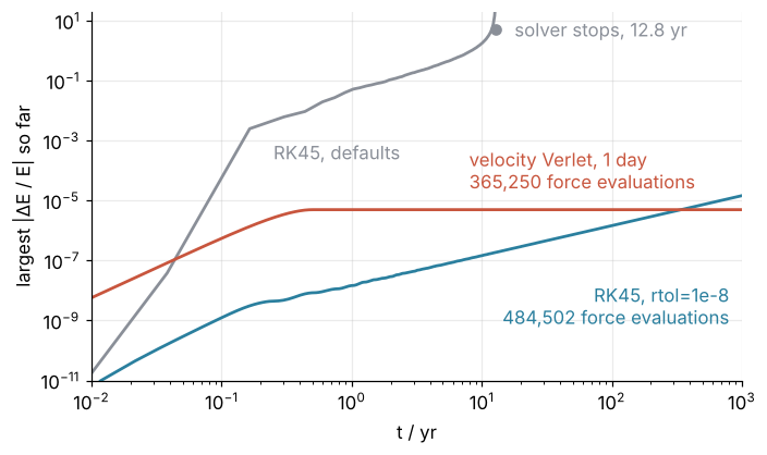
Largest relative energy error so far against time in years, both axes logarithmic, over 1000 years. RK45 at default tolerances passes 100 % and stops at 12.8 years; RK45 at rtol 1e-8 grows in proportion to time; velocity Verlet stays flat at 5e-6.

The tight RK45 rises on a straight line of slope 1 and crosses velocity Verlet's flat line near year 340. For a run of a few decades the tight RK45 is the better integrator, in energy and in position. For a run of millions of orbits, or of molecular collisions, it is not.

Pitfalls

Counting steps instead of force evaluations. Step 2's tight RK45 took 74,502 steps, a fifth of velocity Verlet's 365,250, which makes it look cheap. But RK45 evaluates the force six times per step (it has seven stages, and the last is reused as the first of the next step), plus the rejected steps, for 484,502 evaluations in all. The force is where the time goes in any real simulation, so compare nfev with the number of Verlet steps, as the figure's labels do.

Tightening rtol and expecting the drift to go away. Tighter tolerances move the error line down; they do not flatten it. Over 10 and 100 years:

for rtol in [1e-6, 1e-7, 1e-8, 1e-9, 1e-10]:
    s = solve_ivp(rhs, (0, 100), y0, rtol=rtol, atol=rtol * 1e-3)   # atol small enough that rtol sets the accuracy
    err = np.abs(energy(s.y[:2].T, s.y[2:].T) / E0 - 1)
    print(f"rtol = {rtol:.0e}   nfev = {s.nfev:6d}   energy error"
          f" after 10 yr {err[s.t <= 10].max():.1e}, after 100 yr {err.max():.1e}")

rtol = 1e-06   nfev =  19964   energy error after 10 yr 1.9e-05, after 100 yr 1.9e-04
rtol = 1e-07   nfev =  31574   energy error after 10 yr 5.8e-07, after 100 yr 5.8e-06
rtol = 1e-08   nfev =  48464   energy error after 10 yr 1.5e-07, after 100 yr 1.5e-06
rtol = 1e-09   nfev =  75536   energy error after 10 yr 1.8e-08, after 100 yr 1.8e-07
rtol = 1e-10   nfev = 118118   energy error after 10 yr 1.8e-09, after 100 yr 1.8e-08

Each decade of rtol buys about a decade of accuracy for about 1.5 times the evaluations, and every one of these errors is ten times larger at 100 years than at 10. Whatever you pay, a long enough run eats it.

A step too large for the closest approach. Halley's comet has \(a = 17.83\) AU and \(e = 0.967\), and passes the Sun at 0.59 AU. Start it at aphelion and run one orbit, 75 years:

a_h, e_h = 17.83, 0.967
r_h = np.array([-a_h * (1 + e_h), 0.0])
v_h = np.array([0.0, -np.sqrt(GM * (1 - e_h) / (a_h * (1 + e_h)))])
E_h = energy(r_h, v_h)
r_p = a_h * (1 - e_h)
print(f"tau = r/v at perihelion: {r_p / np.sqrt(GM * (1 + e_h) / r_p) * 365.25:.0f} days")
for days in [10, 1, 0.1]:
    rc, vc = verlet(accel, r_h, v_h, days * DAY, round(a_h**1.5 * 365.25 / days))
    err = np.abs(energy(rc, vc) / E_h - 1)
    print(f"dt = {days:4.1f} days   largest energy error {err.max():.1e}"
          f"  at r = {np.linalg.norm(rc[err.argmax()]):.2f} AU")

tau = r/v at perihelion: 19 days
dt = 10.0 days   largest energy error 1.0e+00  at r = 0.60 AU
dt =  1.0 days   largest energy error 1.1e-02  at r = 0.59 AU
dt =  0.1 days   largest energy error 1.1e-04  at r = 0.59 AU

At 10 days the energy error is 100 %, at 1 day 1 %, both at perihelion. The cause is \(\tau\): \(r/v\) at perihelion is 19 days, so a day is \(\tau/19\), where for the Earth it was \(\tau/56\). The error collects where the orbit bends hardest. The fix is the last rule of Step 4: for an error of 10⁻⁴, \(\Delta t = 1\,\text{day}\cdot\sqrt{10^{-4}/10^{-2}} = 0.1\) day, and the run confirms it.

Variations

A Lennard-Jones pair, the molecular dynamics case. Swap accel for the Lennard-Jones force in reduced units and leave the loop alone; \(\Delta t\) comes from Step 4 with \(\tau = \sigma/v\) at the closest approach.
Adaptive steps break the bounded error. The shadow energy of Step 3 depends on \(\Delta t\), so a step that changes every time switches to a different shadow energy each time, and the error drifts again. That is why molecular dynamics codes keep \(\Delta t\) fixed.
The whole solar system with REBOUND, one of the widely used N-body packages, and its WHFast integrator, built for exactly this job. A tutorial on it is planned.
More bodies. accel_bodies costs \(N^2\) per step; the Barnes-Hut algorithm cuts it to \(N \log N\).

Cheat sheet

a = accel(r)                                   # once, before the loop; r, v updated in place
for k in range(n):
    v += 0.5 * dt * a                          # half kick
    r += dt * v                                # drift
    a = accel(r)                               # the one force evaluation per step
    v += 0.5 * dt * a                          # half kick, its force reused next step
# check: |E/E0 - 1| bounded and flat; growing means a bug or an adaptive step
# dt: tau = r/v at closest approach, start at tau/50, halving must cut the error by 4
# then dt_new = dt * sqrt(tolerable_error / measured_error)