Find where sampled data cross a level: a peak's full width at half maximum

The problem

You have a curve as samples and want the x values where it crosses a level: the edges of a spectral line or a beam profile, the moment a signal passes a threshold. The nearest sample is off by up to half a spacing. Instead, find where y minus the level changes sign and put a straight line through the two samples around it, in plain NumPy. The example is the full width at half maximum (FWHM) of an absorption line, its width at half its height above the baseline: a Gaussian with σ = 2.0 nm and a true FWHM of 4.71 nm, sampled every 0.5 nm and every 2.0 nm. Swap in your own x, y, and level.

The code

Copy

import numpy as np
import matplotlib.pyplot as plt

# ---- data: replace x, y, and EDGE with your own
rng = np.random.default_rng(2)
x = np.arange(630.0, 675.01, 0.5)                              # wavelength, nm
y = (0.10 + 0.004 * (x - 630)                                  # sloping baseline
     + 0.8 * np.exp(-(x - 652.3) ** 2 / (2 * 2.0 ** 2))        # the line, sigma = 2.0 nm
     + 0.015 * rng.standard_normal(x.size))                    # a dip (transmittance) goes in as -y
EDGE = 5.0                       # baseline window at each end, in units of x; must hold no peak
TRUE_FWHM = 2 * np.sqrt(2 * np.log(2)) * 2.0                   # only for the comparison

# ---- level crossings
def crossings(x, y, level):
    s = y - level
    above = s > 0                # a sample exactly on the level is not above: its crossing is found once
    i = np.nonzero(np.diff(above))[0]                          # last sample before each change
    xc = x[i] + s[i] / (s[i] - s[i + 1]) * (x[i + 1] - x[i])   # straight line, solved for the level
    xn = np.where(abs(s[i]) < abs(s[i + 1]), x[i], x[i + 1])   # the nearer sample, for comparison
    return xc, xn

# ---- baseline, level, width
def fwhm(x, y, edge):
    left, right = x < x[0] + edge, x > x[-1] - edge
    x0, x1, y0, y1 = x[left].mean(), x[right].mean(), y[left].mean(), y[right].mean()
    peak = y - (y0 + (y1 - y0) * (x - x0) / (x1 - x0))        # line through the two end means
    level = 0.5 * peak.max()
    xc, xn = crossings(x, peak, level)
    return peak, level, xc, xn, xc[-1] - xc[0], xn[-1] - xn[0]  # outermost pair

# ---- report and plot
print(f"{'spacing':>9s}  {'crossings':>9s}  {'interpolated':>12s}  {'nearest':>8s}  {'true':>7s}")
fig, axes = plt.subplots(2, 1, figsize=(7, 4.4), dpi=110, sharex=True)
for ax, (dx, xs, ys) in zip(axes, [(0.5, x, y), (2.0, x[::4], y[::4])]):
    peak, level, xc, xn, width, width_n = fwhm(xs, ys, EDGE)
    print(f"{dx:6.1f} nm  {xc.size:9d}  {width:9.2f} nm  {width_n:5.2f} nm  {TRUE_FWHM:4.2f} nm")
    for edge in 652.3 + np.array([-0.5, 0.5]) * TRUE_FWHM:   # true half-maximum positions
        ax.axvline(edge, color="#8a8f98", ls="--", lw=1)
    ax.axhline(level, color="#2a7f9e", lw=1.0)
    ax.plot(xs, peak, "o-", color="#1f2a44", ms=4 if dx < 1 else 5, lw=1.0)
    ax.plot(xc[[0, -1]], [level, level], "o-", color="#c8553d", ms=6, lw=1.8)
    ax.plot(xn, np.interp(xn, xs, peak), "o", ms=9, mfc="none", mec="#1f2a44", zorder=3)
    for k, (label, color) in enumerate([(f"Δx = {dx} nm", "#1f2a44"),
            (f"interpolated {width:.2f} nm", "#c8553d"), (f"nearest {width_n:.2f} nm", "#1f2a44"),
            (f"true {TRUE_FWHM:.2f} nm", "#8a8f98")]):      # colored like the marks they name
        ax.text(0.01, 0.98 - 0.12 * k, label, transform=ax.transAxes, va="top", color=color)
    ax.spines[["top", "right"]].set_visible(False)
    ax.set(ylim=(-0.08, 1.0))                                  # room for the text above the level
axes[1].set(xlim=(641.2, 663.8), xlabel="λ / nm")
fig.supylabel("absorbance above baseline", fontsize=11)
plt.show()

  spacing  crossings  interpolated   nearest     true
   0.5 nm          2       4.75 nm   4.50 nm  4.71 nm
   2.0 nm          2       4.84 nm   4.00 nm  4.71 nm

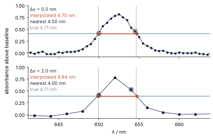
For your own data, replace x and y, set EDGE in your units of x (degrees 2θ, seconds, kelvin) so that both end windows hold only baseline, and pass -y for a dip, since fwhm takes the maximum. np.diff of a boolean array is True where two neighbors differ, not a step of +1 or −1, and np.nonzero returns one index array per dimension, hence the [0].

The knobs

Half the maximum is a convention, and the 0.5 in fwhm is the only place it lives: a laser beam's 1/e² diameter uses 0.135 instead. For a threshold, call crossings with the threshold itself, and add i = i[s[i] <= 0] after the line that finds i to keep only upward crossings. With a formula instead of samples, the crossing is a root for brentq.

The nearest-sample width is a whole number of spacings, so it can never be 4.71 nm: it comes out 4.50 nm and 4.00 nm, while interpolation gives 4.75 nm and 4.84 nm. The coarse grid, every fourth sample, puts 2.4 samples across the FWHM, and without noise it still gives 4.89 nm, 0.18 nm too wide, so noise is not its main error. The chord, the straight line between two samples, cuts across the curved flank and adds 0.13 nm; no sample lands on the top, so the level comes out low and the crossings move outward by another 0.05 nm. With the top sample half a spacing from the center the level would be 12 % low and the width 0.41 nm too large. Below about five samples across the FWHM, the absorption line needs a model, and that is curve fitting.

The width you measure is not the width of the line. A spectrometer smears each wavelength over its resolution width, and when line and smear are both Gaussian the widths add in quadrature: a 3 nm line seen at 2 nm resolution measures √(3² + 2²) = 3.6 nm. Smoothing does the same on purpose. A moving average of n samples is a box whose variance, (n² − 1) Δx²/12, adds to σ², so a 5-sample window at 0.5 nm turns 4.71 nm into 5.0 nm; the operation is a convolution.

Noise moves each crossing by about the noise divided by the Gaussian's slope at half maximum, 0.8 × 0.5 × √(2 ln 2)/σ = 0.235 per nm, so noise of 0.015 moves each edge by about 0.06 nm. For many peaks at once, scipy.signal.peak_widths does the same interpolation after find_peaks, at a fraction of each peak's prominence (its height above the surrounding signal), and returns widths in samples, not in units of x. The find_peaks tutorial shows both.

Pitfalls

Extra crossings from noise. More than two crossings in the printed count means the curve wanders back and forth across the level where it is nearly flat: a level close to the baseline, a flat-topped peak, a noisy shoulder. On this spectrum a level at 3 % of the maximum gives 8 crossings instead of 2. The code keeps the outermost pair, which is right for a single peak, but read the count anyway, and smooth only if you accept the widening from The knobs. Several peaks need find_peaks first, or a crop of x and y around one peak with baseline at both ends, so that each gets its own stretch of data.

Forgetting the baseline. Take half the raw maximum and the level counts the baseline under the peak, 0.19 here, as part of the line. It then sits only 0.31 above the local baseline instead of 0.40, and the width comes out 5.52 nm instead of 4.75 nm. On a sloping baseline the two flanks are also cut at different heights above it, so the edges are lopsided and the center shifts. Subtract the baseline before you set the level, from end windows (EDGE) that hold no line signal.

A crossing exactly on a sample. Integer counts and clipped detector values land on the level more often than you would expect. With np.diff(np.sign(s)), a sample where s is 0 gives two sign changes, −1 to 0 and 0 to +1, so one crossing is counted twice; with strict tests on both sides, s[:-1] < 0 and s[1:] > 0, it is not counted at all. The single boolean s > 0 in the cell treats a sample on the level as below it, so the crossing is found once and lands on that sample.