Convolution: how a small kernel blurs, sharpens, and finds edges (Python)

The question

Here is a test image of 96 × 96 pixels: a bright disk 18 px in radius and a dimmer horizontal bar on a dark background, with noise of standard deviation 0.08 over everything. Beside it are three versions of the same image. Each was made by a convolution with a different kernel, and each kernel is a grid of 3 × 3 numbers, nothing more.

Show code

import numpy as np
import matplotlib.pyplot as plt
from scipy import ndimage as ndi

plt.rcParams.update({
    "figure.figsize": (7, 3.6), "figure.dpi": 110,
    "axes.spines.top": False, "axes.spines.right": False,
    "axes.grid": True, "grid.alpha": 0.25,
    "font.size": 11, "lines.linewidth": 1.8,
})
INK, ACCENT, SECOND, MUTED = "#1f2a44", "#c8553d", "#2a7f9e", "#8a8f98"

# The image is synthetic, so that every edge position and step height is known.
rng = np.random.default_rng(42)
N = 96
rows, cols = np.indices((N, N))
clean = np.full((N, N), 0.2)                                   # background
clean[(rows - 40) ** 2 + (cols - 36) ** 2 <= 18 ** 2] = 1.0    # disk, center row 40, column 36
clean[64:72, 20:84] = 0.7                                      # bar, rows 64 to 71
img = clean + rng.normal(0, 0.08, (N, N))

box = np.full((3, 3), 1 / 9)
gauss = np.array([[1, 2, 1], [2, 4, 2], [1, 2, 1]]) / 16
sharpen = np.array([[0, -1, 0], [-1, 5, -1], [0, -1, 0]], dtype=float)
sobel_x = np.array([[1, 0, -1], [2, 0, -2], [1, 0, -1]], dtype=float)
sobel_y = sobel_x.T

GRAY = dict(cmap="gray", vmin=0, vmax=1.2)
SIGNED = dict(cmap="RdBu_r", vmin=-3.5, vmax=3.5)

fig, axes = plt.subplots(1, 4, figsize=(8, 2.5))
panels = [("image", img, GRAY),
          ("blur", ndi.convolve(img, gauss), GRAY),
          ("sharpen", ndi.convolve(img, sharpen), GRAY),
          ("edges", ndi.convolve(img, sobel_x), SIGNED)]
for ax, (name, im, style) in zip(axes, panels):
    ax.imshow(im, **style)
    ax.text(0.5, -0.04, name, transform=ax.transAxes, ha="center", va="top")
    ax.set_axis_off()
plt.tight_layout()
plt.show()

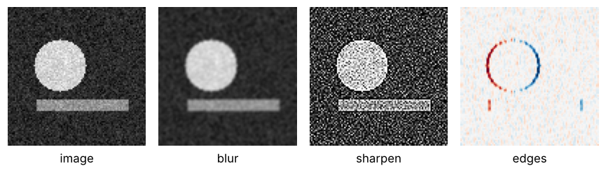
A noisy test image with a bright disk and a horizontal bar, and three versions of it, each made with one 3 × 3 kernel: blurred, sharpened, and an edge map in which the disk's left side is red, its right side blue, and the bar's long edges are missing.

Three things are plain. The blurred version is smoother: the grain of the noise is gone and the outlines have gone soft. The sharpened one is grainier than the original, yet its outlines look crisper. The edge map keeps only outlines, and only some of them: the disk's left side is red, its right side blue, and the long top and bottom edges of the bar are missing. The colormap is RdBu_r, red where brightness rises from left to right, blue where it falls, white where nothing changes.

Less plain is why. All three came out of the same operation, and the only thing that differs is nine numbers. Which property of those nine numbers decides whether you get a blur, a sharper picture, or a map of edges, and can you tell before you run anything? The image is synthetic, so every edge position and step height is known and every answer below can be checked against it. Each picture is one call, ndi.convolve(img, kernel) from scipy.ndimage; what that call computes is the subject here.

The idea: a weighted average that slides

Lay the 3 × 3 grid over a pixel, its center weight on the pixel and the other eight weights on the eight neighbors. Multiply each pixel by the weight on top of it, add the nine products, and write the sum into the output image at the center position. Then move one pixel along and repeat. The grid is the kernel, and the whole sweep is the convolution of the image with that kernel.

One convention belongs to the mechanism from the start: convolution lays the grid down rotated by half a turn, so its top row lands at the bottom and its left column at the right. The box kernel, nine weights of 1/9, looks the same rotated, so the turn changes nothing yet.

With the box kernel the output is the plain average of a pixel and its neighbors. Here is one by hand, at row 40, column 54, on the disk's right edge; the slice takes rows 39 to 41 and columns 53 to 55:

patch = img[39:42, 53:56]
print(patch.round(2))
print(f"box average = {patch.mean():.2f}")

[[0.92 0.27 0.2 ]
 [0.92 1.05 0.07]
 [0.93 0.22 0.12]]
box average = 0.52

The left column lies inside the disk, near 0.92. The right two lie in the background near 0.2, except the center pixel, 1.05, the last of the disk in its row. The average is 0.52, halfway between background and disk: the edge pixel no longer knows which side it belongs to.

Move the window and the average follows whatever is under it: 0.20 in the background, 0.52 on the edge, 0.98 inside the disk.

Show code

from matplotlib.patches import Rectangle
from matplotlib.colors import to_rgba

r0, c0 = 32, 42                                   # top-left corner of the crop
crop = img[r0:r0 + 17, c0:c0 + 21]
fig, axes = plt.subplots(1, 3, figsize=(7.5, 2.8))
for ax, col, where in zip(axes, [60, 54, 46], ["background", "edge", "inside"]):
    ax.imshow(crop, interpolation="nearest", **GRAY)
    ax.add_patch(Rectangle((col - 1 - c0 - 0.5, 40 - 1 - r0 - 0.5), 3, 3,
                           fill=False, edgecolor=SECOND, lw=2.5))
    value = img[39:42, col - 1:col + 2].mean()
    ax.text(0.5, -0.04, f"{where}: {value:.2f}", transform=ax.transAxes, ha="center", va="top")
    ax.set_axis_off()
plt.tight_layout()
plt.show()

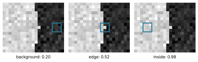
A 3 × 3 window at three positions across the right edge of the disk: in the background, on the edge, inside the disk. The box-kernel averages are 0.20, 0.52, and 0.98, so the edge pixel lands halfway.

A sharp step becomes a ramp three pixels wide, and the noise, averaged over nine pixels, shrinks. Here is that blur one pixel at a time:

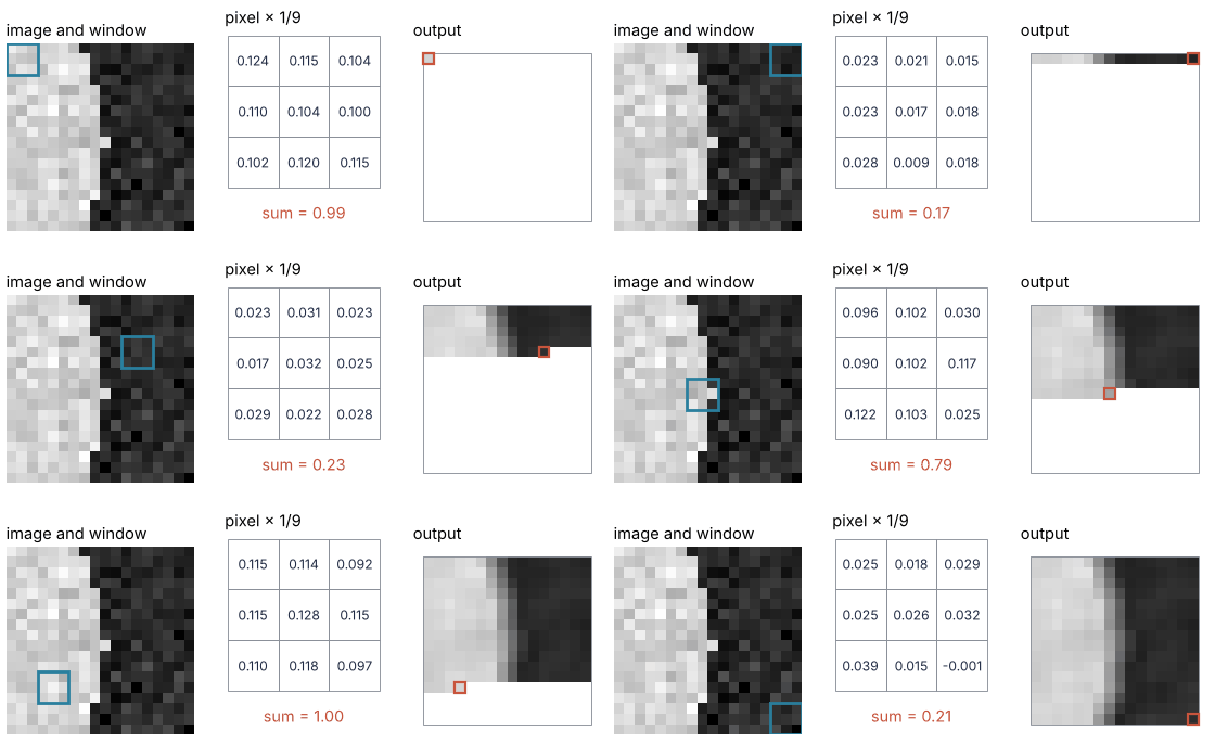
Animation: a 3 × 3 window slides over a crop of the disk edge; at each stop the nine products and their sum are shown, and the sum fills one pixel of the output. Watch the output turn mid-gray where the window straddles the edge.

How I built this: each frame moves the window one step and writes its sum into the output with Matplotlib's FuncAnimation, the technique of Matplotlib animation with FuncAnimation: a probe sweep as a small GIF; the source is animations/kernel-slide/scene.py.

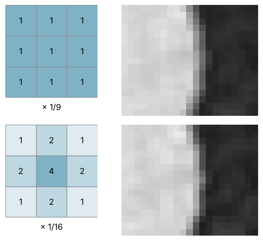
The weights need not be equal. The 3 × 3 Gaussian kernel gives the center pixel 4/16, its four direct neighbors 2/16 each, and the four corners 1/16. Both kernels blur, and the Gaussian blurs the edges less, because it trusts the center pixel more:

Show code

def draw_kernel(ax, weights, factor=""):
    """The kernel as a 3 × 3 tile in SECOND, the window's color: shade by size, negative weights hatched."""
    big = np.abs(weights).max()
    for (i, j), w in np.ndenumerate(weights):
        ax.add_patch(Rectangle((j, i), 1, 1, facecolor=to_rgba(SECOND, 0.6 * abs(w) / big), lw=0))   # zero stays empty
        if w < 0:
            ax.add_patch(Rectangle((j, i), 1, 1, fill=False, hatch="///", edgecolor=SECOND, lw=0))
        ax.add_patch(Rectangle((j, i), 1, 1, fill=False, edgecolor=MUTED, lw=0.8))
        ax.text(j + 0.5, i + 0.5, f"{w:g}", ha="center", va="center",
                bbox=dict(boxstyle="round,pad=0.15", facecolor="white", edgecolor="none") if w < 0 else None)
    if factor:
        ax.text(1.5, 3.15, factor, ha="center", va="top")
    ax.set(xlim=(0, 3), ylim=(3.6, 0), aspect="equal")
    ax.set_axis_off()

fig, axes = plt.subplots(2, 2, figsize=(5.6, 4.6), width_ratios=[0.8, 1])
for row, (weights, factor, kernel) in zip(axes, [(np.ones((3, 3)), "× 1/9", box),
                                                 (gauss * 16, "× 1/16", gauss)]):
    draw_kernel(row[0], weights, factor)
    out = ndi.convolve(img, kernel)[r0:r0 + 17, c0:c0 + 21]     # the crop of the previous figure
    row[1].imshow(out, interpolation="nearest", **GRAY)
    row[1].set_axis_off()
plt.tight_layout()
plt.show()

The box kernel, nine weights of 1/9, and the 3 × 3 Gaussian, weights 1 2 1 / 2 4 2 / 1 2 1 over 16, each beside its output on the pixel crop of the disk's right edge from the previous figure. Both smooth the noise; the box spreads the edge into a wider gray ramp.

The name comes from the bell curve \(e^{-r^2/2\sigma^2}\), where \(r\) is the distance from the center in pixels and \(\sigma\) the width of the bell. Every row and column of the kernel is a multiple of 1, 2, 1. Read as the weights 1/4, 2/4, 1/4 at offsets −1, 0, 1, which sum to 1 like probabilities, they have a standard deviation of 0.71 px: as wide as a bell with \(\sigma = 0.71\) px, though not that bell's values. A wider bell needs more pixels, and scipy.ndimage.gaussian_filter builds the kernel for any \(\sigma\), cut off at \(4\sigma\) on either side. Filter an image that is zero except for one pixel of 1, and each output pixel picks up a single weight: the output is the kernel itself.

offsets, w = np.array([-1, 0, 1]), np.array([1, 2, 1]) / 4
print(f"1-2-1 kernel: sigma = {np.sqrt(np.sum(w * offsets**2)):.2f} px")

delta = np.zeros((61, 61))
delta[30, 30] = 1.0                               # a single bright pixel shows the kernel itself
for sigma in [1.5, 3]:
    size = np.count_nonzero(ndi.gaussian_filter(delta, sigma)[30])
    print(f"gaussian_filter, sigma = {sigma} px: kernel {size} × {size}")

1-2-1 kernel: sigma = 0.71 px
gaussian_filter, sigma = 1.5 px: kernel 13 × 13
gaussian_filter, sigma = 3 px: kernel 25 × 25

At \(\sigma = 3\) px that is 625 weights instead of nine.

Negative weights: sharpening and edges

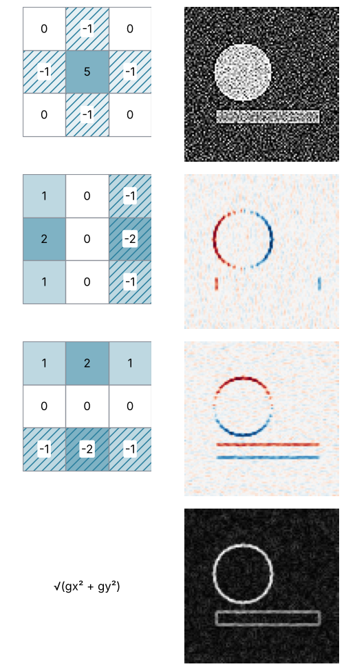
The sharpening kernel has 5 in the center and −1 on the four direct neighbors. Split the 5 as 1 + 4 and it reads: the pixel, plus four times the pixel minus its four neighbors. It is symmetric, so the turn does not matter. On a flat region the second part is zero and the pixel comes out unchanged. At an edge it overshoots: on row 40 the last disk pixel comes out at 3.77 where the disk is 1.0, the first background pixel at −1.09 where the background is 0.2. The eye reads that overshoot as a crisper outline.

The Sobel x kernel is written with a column of 1, 2, 1 on the left, zeros in the middle, and −1, −2, −1 on the right. Here the turn matters. Rotated by half a turn, the positive column lands on the right, so what is applied is the right column minus the left column, weighted 1, 2, 1 down the rows, which is zero on a flat region. Across a vertical step of 0.8, from the background at 0.2 to the disk at 1.0, it is (1 + 2 + 1) × 0.8 = 3.2: positive where brightness rises to the right, negative where it falls. Sobel y, sobel_x.T, applies the row below minus the row above, positive where brightness rises down the image. The bar is a step of 0.5, so Sobel y predicts (1 + 2 + 1) × 0.5 = 2.0 at its edges:

gx = ndi.convolve(img, sobel_x)
gy = ndi.convolve(img, sobel_y)
print(f"Sobel x, row 40:   left edge (col 18) {gx[40, 18]:+.2f}   right edge (col 54) {gx[40, 54]:+.2f}")
print(f"Sobel y, col 50:   bar top (row 64)   {gy[64, 50]:+.2f}   bar bottom (row 71) {gy[71, 50]:+.2f}")

Sobel x, row 40:   left edge (col 18) +3.12   right edge (col 54) -3.22
Sobel y, col 50:   bar top (row 64)   +1.87   bar bottom (row 71) -2.00

Measured against predicted: +3.12 and −3.22 against 3.2, +1.87 and −2.00 against 2.0. The misses are the noise.

One kernel sees one direction. Along a horizontal edge the left and right columns of the window hold the same values, so Sobel x returns zero there; that is why the bar's long edges were missing from the first figure. An outline in every direction takes two kernels, combined pixel by pixel as \(\sqrt{g_x^2 + g_y^2}\) from their outputs \(g_x\) and \(g_y\):

Show code

fig, axes = plt.subplots(4, 2, figsize=(5, 9), width_ratios=[0.8, 1])
magnitude = np.hypot(gx, gy)
results = [(sharpen, ndi.convolve(img, sharpen), GRAY),
           (sobel_x, gx, SIGNED),
           (sobel_y, gy, SIGNED),
           (None, magnitude, dict(cmap="gray", vmin=0, vmax=4))]
for row, (kernel, out, style) in zip(axes, results):
    if kernel is None:
        row[0].text(0.5, 0.5, "√(gx² + gy²)", ha="center", va="center", transform=row[0].transAxes)
        row[0].set_axis_off()
    else:
        draw_kernel(row[0], kernel)
    row[1].imshow(out, **style)
    row[1].set_axis_off()
plt.tight_layout()
plt.show()

Sharpen, Sobel x, and Sobel y kernels beside their outputs, and the combined edge magnitude. Sobel x marks the disk's left and right sides in red and blue, Sobel y the top and bottom of the disk and bar; only their combination outlines everything.

Row 40, through the middle of the disk, shows the numbers:

Show code

fig, axes = plt.subplots(3, 1, figsize=(7, 6), sharex=True)
for ax, (name, kernel) in zip(axes, [("Gaussian", gauss), ("sharpen", sharpen), ("Sobel x", sobel_x)]):
    ax.plot(img[40], color=INK, lw=1.2)
    ax.plot(ndi.convolve(img, kernel)[40], color=ACCENT)
    for edge in [17.5, 54.5]:
        ax.axvline(edge, color=MUTED, lw=1, ls="--")
    ax.text(94, 0.95, "row 40", color=INK, transform=ax.get_xaxis_transform(), ha="right", va="top")   # direct labels
    ax.text(94, 0.72, f"after {name}", color=ACCENT, transform=ax.get_xaxis_transform(), ha="right", va="top")
    ax.set_ylabel("brightness / a.u.")
axes[2].annotate(f"{gx[40, 18]:+.2f}", (18, gx[40, 18]), xytext=(6, -4), textcoords="offset points", va="top")
axes[2].annotate(f"{gx[40, 54]:+.2f}", (54, gx[40, 54]), xytext=(6, 4), textcoords="offset points")
axes[2].set(xlabel="column / px", xlim=(0, 95))
plt.tight_layout()
plt.show()

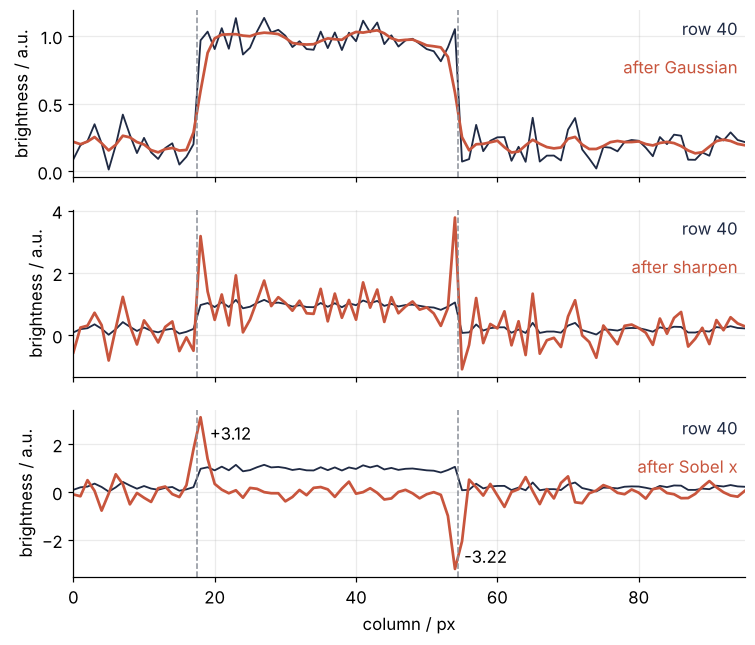
Brightness along row 40 against column in px, before and after three kernels. The Gaussian rounds the steps at columns 18 and 54, sharpen overshoots on both sides of each, and Sobel x is near 0 except a spike of +3.12 at the left edge and -3.22 at the right.

The Gaussian turns both steps into ramps, sharpen overshoots on both sides of each, and Sobel x stays near zero except for one spike per edge. Over the flat background, though, the Sobel trace wobbles by a few tenths, several times more than the original row. The kernel amplified the noise, by an amount you can predict.

Formalization

Written out, the output at pixel \((i, j)\) is

\[(g * k)[i, j] = \sum_{m=-1}^{1} \sum_{n=-1}^{1} g[i - m,\, j - n]\; k[m, n] ,\]

with \(g\) the image and \(k\) the kernel, indexed from its center at \(m = n = 0\). A kernel of \((2r+1) \times (2r+1)\) weights runs \(m\) and \(n\) from \(-r\) to \(r\). The minus signs are the half turn of the previous sections: the weight at the kernel's top left, \(m = n = -1\), multiplies the pixel at the bottom right of the window. The same sum with plus signs is called correlation, and SciPy has both:

Show code

print(f"Sobel x at (40, 54):  convolve {ndi.convolve(img, sobel_x)[40, 54]:+.2f}   "
      f"correlate {ndi.correlate(img, sobel_x)[40, 54]:+.2f}")

Sobel x at (40, 54):  convolve -3.22   correlate +3.22

Same kernel, same pixel, opposite sign. The turn is the convention because it makes convolution commutative, image and kernel interchangeable, and turns it into a plain multiplication under the Fourier transform, the subject of The Fourier transform: asking a signal how much of each frequency it contains.

At the border part of the window hangs over the edge of the image, and what it finds there is a choice, not a fact. With zeros (mode="constant") the Gaussian pulls the mean of the top row from 0.198 down to 0.148, a quarter lower, since a quarter of its weight lies in the overhanging row. With mode="reflect", the default in scipy.ndimage, the image is mirrored at its edge and the row stays at 0.198. Keep the default unless you have a reason; zeros draw a dark frame around every result.

Show code

print(f"top row mean:  image {img[0].mean():.3f}   "
      f"constant {ndi.convolve(img, gauss, mode='constant')[0].mean():.3f}   "
      f"reflect {ndi.convolve(img, gauss)[0].mean():.3f}")

top row mean:  image 0.198   constant 0.148   reflect 0.198

The sum of the weights. A flat region of brightness \(b\) comes out as \(b\) times the sum of the weights, because every weight multiplies the same \(b\). Sum 1 keeps brightness: the image mean of 0.315 comes out as 0.315 under the box, the Gaussian, and sharpen alike. Sum 0 sends a flat region to zero and keeps only change, which is why the mean under Sobel x is −0.001.

Show code

kernels = {"box": box, "Gaussian": gauss, "sharpen": sharpen, "Sobel x": sobel_x}
print(f"image     mean {img.mean():+.3f}")
for name, k in kernels.items():
    print(f"{name:9s} sum {k.sum():3.0f}   mean {ndi.convolve(img, k).mean():+.3f}")

image     mean +0.315
box       sum   1   mean +0.315
Gaussian  sum   1   mean +0.315
sharpen   sum   1   mean +0.315
Sobel x   sum   0   mean -0.001

The squares of the weights. The output at a pixel is \(\sum k[m,n]\,(b + \varepsilon[m,n])\), the brightness under the window plus the noise \(\varepsilon\) of each of the nine pixels. The nine noise values are independent, and the variance of a sum of independent terms is the sum of their variances. Multiplying a term by \(k\) multiplies its variance by \(k^2\). So noise of standard deviation \(s\) comes out as

\[s_\text{out} = s \sqrt{\textstyle\sum k^2} .\]

For the box kernel \(\sum k^2 = 9 \times (1/9)^2 = 1/9\), and the noise drops to \(s/3\): the box output is the mean of nine values, and \(s/3\) is the standard error of that mean, as in The standard error of the mean: why four times the data halves the error. Prediction against measurement in the empty top-right corner, rows 2 to 17 and columns 70 to 93:

Show code

corner = (slice(2, 18), slice(70, 94))
s = img[corner].std()
print(f"noise in the corner: s = {s:.3f}\n")
print("kernel     sum k²   factor   predicted   measured")
for name, k in kernels.items():
    factor = np.sqrt(np.sum(k**2))
    measured = ndi.convolve(img, k)[corner].std()
    print(f"{name:9s} {np.sum(k**2):7.3f}   {factor:6.3f}   {s * factor:9.3f}   {measured:8.3f}")

noise in the corner: s = 0.083

kernel     sum k²   factor   predicted   measured
box         0.111    0.333       0.028      0.029
Gaussian    0.141    0.375       0.031      0.033
sharpen    29.000    5.385       0.449      0.426
Sobel x    12.000    3.464       0.289      0.303

Prediction and measurement agree to within 7 %, which is what 384 pixels of noise allow. Sharpen multiplies the noise by \(\sqrt{29} = 5.4\), and that is the grain of the first figure. Sobel x multiplies it by \(\sqrt{12} = 3.5\), the wobble on the profile.

The same rule says why you blur before looking for edges. A blur divides the noise by its factor everywhere, while a step keeps its full height and only spreads over a few more pixels, so the Sobel spike loses less than the noise does. After gaussian_filter with \(\sigma = 1.5\) px the edge magnitude at the disk's right edge falls from 3.22 to 1.49, but the median magnitude in the empty corner falls from 0.37 to 0.07:

Show code

def edges(image):
    return np.hypot(ndi.convolve(image, sobel_x), ndi.convolve(image, sobel_y))

for name, image in [("raw", img), ("blurred, sigma 1.5 px", ndi.gaussian_filter(img, 1.5))]:
    mag = edges(image)
    edge, background = mag[40, 54], np.median(mag[corner])
    print(f"{name:22s} edge {edge:.2f}   background {background:.2f}   ratio {edge / background:4.1f}")

raw                    edge 3.22   background 0.37   ratio  8.8
blurred, sigma 1.5 px  edge 1.49   background 0.07   ratio 21.9

The edge stood 9 times above the background before the blur and stands 22 times above it after.

Separability. The 3 × 3 Gaussian is the outer product of [1, 2, 1]/4 with itself: every entry of the column times every entry of the row, so the corner is 1/4 × 1/4 = 1/16 and the center 2/4 × 2/4 = 4/16. Sobel x is the outer product of [1, 2, 1] down the rows, a smoothing, and [1, 0, −1] across, a difference. A kernel built this way can be applied as two 1D passes, down the columns and then along the rows, with the same result. For the 25 × 25 Gaussian of \(\sigma = 3\) px that is 625 multiplications per pixel against 50:

Show code

x = np.arange(-12, 13)                            # radius 12 = 4 sigma for sigma = 3 px
g1 = np.exp(-x**2 / (2 * 3.0**2))
g1 /= g1.sum()
full = ndi.convolve(img, np.outer(g1, g1))        # one pass with the 25 × 25 kernel
two_pass = ndi.convolve1d(ndi.convolve1d(img, g1, axis=0), g1, axis=1)
print(f"multiplications per pixel: {g1.size**2} (2D) against {2 * g1.size} (two 1D passes)")
print(f"2D against two passes:      max difference {np.abs(full - two_pass).max():.1e}")
print(f"gaussian_filter(img, 3):    max difference {np.abs(full - ndi.gaussian_filter(img, 3)).max():.1e}")

multiplications per pixel: 625 (2D) against 50 (two 1D passes)
2D against two passes:      max difference 2.4e-15
gaussian_filter(img, 3):    max difference 2.4e-15

The three agree to rounding. gaussian_filter works this way internally, which is why a wide Gaussian costs little.

See it in code

Everything above used scipy.ndimage.convolve. Here is the sum of the formalization as a plain double loop, with the image mirrored at its edge the way mode="reflect" does it, set against the library and against ndi.sobel:

Show code

def convolve_by_hand(image, kernel):
    padded = np.pad(image, 1, mode="symmetric")   # NumPy's name for SciPy's "reflect"
    turned = kernel[::-1, ::-1]                    # the half turn
    out = np.empty_like(image)
    for i in range(image.shape[0]):
        for j in range(image.shape[1]):
            out[i, j] = np.sum(padded[i:i + 3, j:j + 3] * turned)
    return out

print(f"loop against ndi.convolve, box:        {np.abs(convolve_by_hand(img, box) - ndi.convolve(img, box)).max():.1e}")
print(f"loop against ndi.convolve, Sobel x:    {np.abs(convolve_by_hand(img, sobel_x) - gx).max():.1e}")
print(f"ndi.sobel(axis=1) against Sobel x:     {np.abs(ndi.sobel(img, axis=1) - gx).max():.1e}")
print(f"ndi.sobel at the disk's right edge:    {ndi.sobel(img, axis=1)[40, 54]:+.2f}")

loop against ndi.convolve, box:        4.4e-16
loop against ndi.convolve, Sobel x:    8.9e-16
ndi.sobel(axis=1) against Sobel x:     8.9e-16
ndi.sobel at the disk's right edge:    -3.22

The library computes exactly the sum of the formalization; the differences are rounding in the last digit. ndi.sobel with axis=1 is the Sobel x kernel of the section on negative weights, with the same sign convention, so it too reads −3.22 at the disk's right edge against the 3.2 that a step of 0.8 predicts. The keyword of ndi.convolve worth knowing is mode, whose default "reflect" mirrors the image at its border.

Where it shows up

Microscopy. A micrograph is the specimen convolved with the point spread function, the blurred spot the microscope makes of a single point of light. Deconvolution tries to compute the specimen back from the blurred image, and the Gaussian smoothing before thresholding in Counting cells with scipy.ndimage: how many are there, and how large? is the blur of this tutorial.
Seismic sections. The convolutional model treats a recorded trace as the reflectivity of the layers convolved with the source wavelet. Gradient kernels run over a stacked section make faults stand out where reflectors break off.
Satellite images and elevation models. Sobel-type gradients on a Landsat band trace coastlines and the calving fronts of glaciers. On a digital elevation model the Sobel output is in meters, eight times the height change per pixel, so dividing by 8 and by the pixel spacing gives the slope.
Spectra. A moving average smooths a Raman or infrared spectrum, and so does a Savitzky-Golay filter, which fits a short polynomial in each window but whose weights come out as one fixed kernel. A measured line is the true line convolved with the instrument function.
Finite differences. The five-point Laplacian of a PDE solver, the stencil with −4 in the center and 1 on the four neighbors, is a kernel with sum 0. Its 1D cousin, the weights 1, −2, 1, is convolved with the string at every time step of The wave equation with leapfrog finite differences: a pulse on a string.
Neural networks. A convolutional layer learns its kernels from training data instead of having them written down. The first layer of a trained image network often ends up with kernels that look like Sobel.

In every case the kernel says what it will do before you run it: a sum of one keeps brightness, a sum of zero finds change, and the sum of the squares says what happens to the noise.

The question

The idea: a weighted average that slides

Negative weights: sharpening and edges

Formalization

See it in code

Where it shows up

Further reading