Band structure with plane waves in NumPy: an electron in a 1D crystal

The problem: where does a crystal forbid an electron's energy?

An electron in a one-dimensional crystal with atoms 3 Å apart feels a potential that ripples with the lattice, \(V(x) = V_0\cos(2\pi x/a)\). A free electron may have any energy. With \(V_0 = 1\) eV this one may not: a range of energies 1 eV wide is forbidden, as nearly-free-electron theory predicts from the ripple alone. That theory treats the potential as small. The question is how far it holds when \(V_0\) grows to 16 eV, nearly four times the 4.18 eV a free electron has when its wavelength is two lattice spacings.

In a box the allowed energies form a discrete ladder. In a crystal, Bloch's theorem (Ashcroft and Mermin, chapter 8) says that each state repeats from one cell to the next up to a phase, \(ka\) per cell, and the wave number \(k\) labels that phase. For each \(k\) there is again a ladder, \(E_1(k) < E_2(k) < \dots\), and as \(k\) varies each rung sweeps out a range of energies, an energy band. Energies that no \(k\) reaches form a gap. A phase of \(ka\) and one of \(ka + 2\pi\) are the same phase, so \(k\) from \(-\pi/a\) to \(\pi/a\) covers every state. That interval is the Brillouin zone, and its ends, \(k = \pm\pi/a\), are the zone boundary.

Write the state as a sum of plane waves and the Schrödinger equation becomes one Hermitian matrix per \(k\), whose eigenvalues are the energies at that \(k\). Diagonalizing it is the job of eigh, as in the normal modes tutorial.

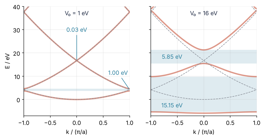
Energy bands for a weak (1 eV) and a strong (16 eV) cosine potential, energy in eV against k/(π/a). The first gap grows from 1.00 to 15.15 eV, and the lowest band flattens to 0.56 eV wide below zero.

On the left the bands hug the dashed free-electron parabola and open narrow gaps; on the right the lowest band is almost flat. Each panel comes from 201 diagonalizations of a 21 × 21 matrix, and the six steps below build it.

Setup

Energies are in eV and lengths in Å throughout, so the one constant of the kinetic energy, \(\hbar^2/2m_e\), is converted once from the SI values in scipy.constants:

import numpy as np
import matplotlib.pyplot as plt
from scipy import constants

C = constants.hbar**2 / (2 * constants.m_e * constants.e) * 1e20   # hbar^2/2m_e in eV Å^2
a = 3.0                  # lattice spacing / Å
G0 = 2 * np.pi / a       # shortest reciprocal lattice vector / Å^-1
K = 10                   # plane waves n = -K ... K, 21 in all

plt.rcParams.update({
    "figure.figsize": (7, 3.6), "figure.dpi": 110,
    "axes.spines.top": False, "axes.spines.right": False,
    "axes.grid": True, "grid.alpha": 0.25,
    "font.size": 11, "lines.linewidth": 1.8,
})
INK, ACCENT, SECOND, MUTED = "#1f2a44", "#c8553d", "#2a7f9e", "#8a8f98"

print(f"hbar^2/2m_e = {C:.3f} eV Å^2,  free energy at k = pi/a: {C * (np.pi / a)**2:.3f} eV")

hbar^2/2m_e = 3.810 eV Å^2,  free energy at k = pi/a: 4.178 eV

Step 1: Turn the Schrödinger equation into a matrix

Multiply a state at wave number \(k\) by \(e^{-ikx}\) and the phase \(ka\) per cell cancels: what is left repeats exactly, so it is a Fourier series in \(G_0 = 2\pi/a\). The state is then a sum of plane waves whose wave numbers differ from \(k\) by multiples of \(G_0\), and the periodic potential is a Fourier series with the same \(G_0\):

\[\psi(x) = \sum_n c_n\, e^{i(k + nG_0)x}, \qquad V(x) = \sum_m V_m\, e^{imG_0x}.\]

The coefficient \(V_m\) is the mean of \(V(x)\,e^{-imG_0x}\) over one cell. Put both into \(-C\psi'' + V\psi = E\psi\), with \(C = \hbar^2/2m_e\). The second derivative multiplies each plane wave by \(-(k + nG_0)^2\), so the kinetic term stays on its own wave. The potential does not: \(V_m e^{imG_0x}\) times \(c_{n'} e^{i(k+n'G_0)x}\) is the plane wave with index \(n = n' + m\). Collect the coefficient of each plane wave and you get one equation per \(n\):

\[C(k + nG_0)^2\, c_n + \sum_{n'} V_{n-n'}\, c_{n'} = E\, c_n .\]

That is a matrix eigenvalue problem: row \(n\), column \(n'\) holds \(V_{n-n'}\), so every diagonal of the matrix holds one Fourier component, and the kinetic energy sits on the main diagonal. The sum runs over all integers, so the matrix is infinite. Keeping \(|n| \le K\) leaves \(2K + 1\) waves. That works because the kinetic diagonal grows as \(n^2\), and waves far up the ladder barely mix with the low states; Step 5 checks it.

The components are needed up to \(|m| = 2K\), since \(n - n'\) runs from \(-2K\) to \(2K\). A cell sampled at 256 points gives them as plain means:

x = np.arange(256) * a / 256          # one cell, the endpoint left out

def fourier_components(V, mmax):
    """V_m for m = -mmax ... mmax, as the cell mean of V(x) exp(-i m G0 x)."""
    m = np.arange(-mmax, mmax + 1)
    return np.exp(-1j * np.outer(m, G0 * x)) @ V / len(x)

V0 = 1.0                              # eV
Vm = fourier_components(V0 * np.cos(G0 * x), 2 * K)
for m in range(-3, 4):
    print(f"V_{m:+d} = {round(Vm[m + 2 * K].real, 4) + 0:+.4f} eV   |imag| = {abs(Vm[m + 2 * K].imag):.0e}")

V_-3 = +0.0000 eV   |imag| = 3e-17
V_-2 = +0.0000 eV   |imag| = 9e-17
V_-1 = +0.5000 eV   |imag| = 2e-18
V_+0 = +0.0000 eV   |imag| = 0e+00
V_+1 = +0.5000 eV   |imag| = 2e-18
V_+2 = +0.0000 eV   |imag| = 9e-17
V_+3 = +0.0000 eV   |imag| = 3e-17

The cosine has 0.5 eV at \(m = \pm 1\) and nothing else beyond rounding. A cosine couples only neighboring plane waves.

Step 2: Build the Hamiltonian for one k

The plane waves are indexed by n from \(-K\) to \(K\), and the matrix element at row \(n\), column \(n'\) is looked up by the difference \(n - n'\), shifted by \(2K\) to land in Vm:

def hamiltonian(k, Vm, K=K):
    n = np.arange(-K, K + 1)
    mmax = (len(Vm) - 1) // 2
    H = Vm[n[:, None] - n[None, :] + mmax]         # V_(n - n') at (n, n')
    return H + np.diag(C * (k + n * G0)**2)

H = hamiltonian(0.0, Vm)
with np.printoptions(precision=3, suppress=True):
    print(np.round(H[K - 1:K + 2, K - 1:K + 2].real, 3) + 0)   # waves n = -1, 0, 1
print("Hermitian:", np.allclose(H, H.conj().T))

[[16.712  0.5    0.   ]
 [ 0.5    0.     0.5  ]
 [ 0.     0.5   16.712]]
Hermitian: True

At \(k = 0\) the waves \(n = \pm 1\) cost 16.71 eV of kinetic energy and \(n = 0\) costs nothing. The 0.5 eV of \(V_{\pm 1}\) sits beside the diagonal, and two steps out there is zero. A real potential has \(V_{-m}\) equal to the complex conjugate of \(V_m\), so \(H\) is Hermitian. eigh takes complex Hermitian matrices as well as the real symmetric ones of the prerequisite.

Step 3: Read off the gaps and check them

Set \(V\) to zero for a moment and \(H\) is diagonal, its eigenvalues the free energies \(C(k + nG_0)^2\), one branch per \(n\). Where two branches meet, the potential couples two waves of equal energy, and a gap opens. At \(k = \pi/a\) the waves \(n = 0\) and \(n = -1\) meet at \(E_\mathrm{f} = C(\pi/a)^2 = 4.18\) eV, coupled by \(V_1\). That 2 × 2 block has the eigenvalues \(E_\mathrm{f} \pm |V_1|\), a first gap of \(2|V_1| = V_0\).

At \(k = 0\) the waves \(n = \pm 1\) meet at \(4E_\mathrm{f}\), but a cosine has no \(V_2\) to couple them. They reach each other only through \(n = 0\), which lies \(4E_\mathrm{f}\) below. Keep just these three waves. In the sine-like state, \(c_{-1} = -c_1\), the two couplings to \(n = 0\) cancel, so it stays at \(4E_\mathrm{f}\). The cosine-like state, \(c_{-1} = c_1\), meets \(n = 0\) with \(\sqrt2\,V_1\) once normalized: a 2 × 2 block with \(4E_\mathrm{f}\) and \(0\) on the diagonal, whose upper eigenvalue \(2E_\mathrm{f} + \sqrt{4E_\mathrm{f}^2 + 2V_1^2}\) lies, once the root is expanded for small \(V_0\), \(V_0^2/8E_\mathrm{f}\) above \(4E_\mathrm{f}\). That is the second gap. The waves \(n = \pm 2\) shift both states alike and leave it unchanged.

np.linalg.eigvalsh is eigh without the eigenvectors: it returns only the energies, in ascending order. Compare both estimates with the full matrix:

E_zb = np.linalg.eigvalsh(hamiltonian(np.pi / a, Vm))
E_0 = np.linalg.eigvalsh(hamiltonian(0.0, Vm))
E_free = C * (np.pi / a)**2                        # free energy at the zone boundary

print(f"first gap  (k = pi/a): {E_zb[1] - E_zb[0]:.5f} eV   first order: {V0:.5f} eV")
print(f"second gap (k = 0)   : {E_0[2] - E_0[1]:.5f} eV   second order: {V0**2 / (8 * E_free):.5f} eV")

first gap  (k = pi/a): 0.99978 eV   first order: 1.00000 eV
second gap (k = 0)   : 0.02987 eV   second order: 0.02992 eV

The matrix agrees with nearly-free-electron theory to 0.02 % at first order and to 0.2 % at second. The second gap is 33 times smaller than the first because the push from a wave 16.71 eV away is the coupling squared over that distance.

Step 4: Sweep k across the Brillouin zone

\(k\) stops at \(\pm\pi/a\) because a phase per cell repeats after \(2\pi\). The free branches \(C(k + nG_0)^2\) of Step 3, dashed below, are pieces of the single free-electron parabola \(E = Cq^2\) with \(q = k + nG_0\): a plane wave \(e^{iqx}\) has the same phase per cell as \(e^{ikx}\), so the parabola is cut into pieces \(2\pi/a\) wide and shifted into the zone. Pieces cross at \(k = \pi/a\), where the waves \(n\) and \(-1-n\) meet, and at \(k = 0\), where \(n\) and \(-n\) meet. By Step 3's argument, each crossing of waves \(n\) and \(n'\) opens a gap of \(2|V_{n-n'}|\) to first order. At the zone boundary \(n - n'\) is odd, at \(k = 0\) even, so gap \(n\) is about \(2|V_n|\) and sits at the zone boundary for odd \(n\), at \(k = 0\) for even \(n\).

The sweep calls eigvalsh once per \(k\) and stacks the results into an array with one row per \(k\). In one dimension only two branches meet at a crossing, and the potential splits them, so the bands never cross and column \(j\) of that array is band \(j\):

def bands(V0, ks):
    Vm = fourier_components(V0 * np.cos(G0 * x), 2 * K)
    return np.array([np.linalg.eigvalsh(hamiltonian(k, Vm)) for k in ks])

def draw_bands(ax, ks, E, nbands=4):
    kk = ks / (np.pi / a)
    for j in range(nbands):
        ax.plot(kk, E[:, j], color=ACCENT, lw=2.6, alpha=0.6)   # wide and light, so the dashes show
    for n in range(-2, 3):                          # free branches, drawn on top of the bands
        ax.plot(kk, C * (ks + n * G0)**2, color=MUTED, ls="--", lw=1)
    ax.set(xlabel="k / (π/a)", xlim=(-1, 1))

ks = np.linspace(-np.pi / a, np.pi / a, 201)
E_weak = bands(1.0, ks)
print("array of energies:", E_weak.shape)

fig, ax = plt.subplots()
draw_bands(ax, ks, E_weak)
ax.set(ylabel="E / eV", ylim=(-1, 40))
ax.annotate(f"{E_weak[-1, 1] - E_weak[-1, 0]:.2f} eV", xy=(1, 4.2), xytext=(0.62, 9),
            color=SECOND, arrowprops=dict(arrowstyle="-", color=SECOND, lw=1))
ax.annotate(f"{E_weak[100, 2] - E_weak[100, 1]:.3f} eV", xy=(0, 16.7), xytext=(0, 30), ha="center",
            color=SECOND, arrowprops=dict(arrowstyle="-", color=SECOND, lw=1))
plt.show()

array of energies: (201, 21)

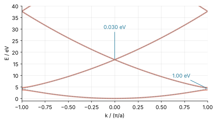
Energy bands of an electron in a 1D crystal with a 1 eV cosine potential, energy in eV against k from −π/a to π/a. Solid: the lowest four bands. Dashed: the free-electron parabola folded into the zone. The bands follow the parabola except where branches cross, where gaps open.

Away from the crossings the bands lie on the dashed parabola. At the crossings they split, by 1.00 eV at the zone boundary and by 0.030 eV at \(k = 0\), too small to see at this scale.

Step 5: Turn up the potential and count plane waves

Repeat Step 3 for 29 values of \(V_0\) from 0.25 to 32 eV and record the first gap over \(V_0\) and the width of the lowest band:

V0s = np.geomspace(0.25, 32, 29)
ratio, width = [], []
for V0 in V0s:
    E = bands(V0, [0.0, np.pi / a])
    ratio.append((E[1, 1] - E[1, 0]) / V0)
    width.append(E[1, 0] - E[0, 0])
ratio, width = np.array(ratio), np.array(width)

for V0, r, w in list(zip(V0s, ratio, width))[::4]:
    print(f"V0 = {V0:6.2f} eV   gap/V0 = {r:.4f}   band 1 width = {w:.3f} eV")
print(f"first-order estimate 1 % off at V0 = {np.interp(0.01, 1 - ratio, V0s):.1f} eV")

V0 =   0.25 eV   gap/V0 = 1.0000   band 1 width = 4.055 eV
V0 =   0.50 eV   gap/V0 = 0.9999   band 1 width = 3.934 eV
V0 =   1.00 eV   gap/V0 = 0.9998   band 1 width = 3.701 eV
V0 =   2.00 eV   gap/V0 = 0.9991   band 1 width = 3.268 eV
V0 =   4.00 eV   gap/V0 = 0.9964   band 1 width = 2.533 eV
V0 =   8.00 eV   gap/V0 = 0.9859   band 1 width = 1.509 eV
V0 =  16.00 eV   gap/V0 = 0.9469   band 1 width = 0.560 eV
V0 =  32.00 eV   gap/V0 = 0.8325   band 1 width = 0.102 eV
first-order estimate 1 % off at V0 = 6.7 eV

The estimate holds to 1 % up to 6.7 eV, 1.6 times the free energy at the zone boundary. Beyond that the gap falls behind \(V_0\) and the lowest band flattens, from 4.06 eV wide to 0.10 eV.

A strong potential mixes more plane waves into each state, so the 21 waves need checking where it is strongest. At \(V_0 = 16\) eV, compare the energies at \(k = \pi/a\) for a few truncations with 61 waves:

def edges(V0, N):
    Kn = (N - 1) // 2
    Vm = fourier_components(V0 * np.cos(G0 * x), 2 * Kn)
    return np.linalg.eigvalsh(hamiltonian(np.pi / a, Vm, K=Kn))

ref = edges(16.0, 61)
for N in [5, 7, 9, 21]:
    err = np.abs(edges(16.0, N) - ref[:N])
    print(f"N = {N:2d}   error of bands 1-{min(N, 7)}:", np.array2string(err[:7], precision=4, suppress_small=True))

err32 = np.abs(edges(32.0, 21)[:10] - edges(32.0, 61)[:10]).max()
print(f"V0 = 32 eV, N = 21: largest error of the lowest ten bands {err32:.0e} eV")

N =  5   error of bands 1-5: [0.01   0.0267 0.269  0.6581 0.6336]
N =  7   error of bands 1-7: [0.     0.0001 0.0027 0.0026 0.0024 0.6322 0.477 ]
N =  9   error of bands 1-7: [0.     0.     0.     0.     0.0005 0.0013 0.0008]
N = 21   error of bands 1-7: [0. 0. 0. 0. 0. 0. 0.]
V0 = 32 eV, N = 21: largest error of the lowest ten bands 2e-12 eV

With seven waves, bands 1 to 5 are within 0.003 eV and bands 6 and 7 are off by 0.6 and 0.5 eV. The top few eigenvalues of any truncation are wrong, because the waves they would mix with were cut. Grow \(N\) until the bands you plot stop moving. With 21 waves the lowest ten bands agree with the 61-wave reference to \(2 \times 10^{-12}\) eV even at 32 eV.

Step 6: Draw the weak and the strong crystal side by side

Call the plotting function from Step 4 for 1 eV and 16 eV, and shade and label the first two gaps:

labels = {1.0: [(0.78, 11.5), (0, 30)], 16.0: [(-0.6, -2.5), (-0.6, 18.4)]}   # where each gap is named
fig, axes = plt.subplots(1, 2, figsize=(8, 3.8), sharey=True)
for ax, V0 in zip(axes, [1.0, 16.0]):
    E = bands(V0, ks)
    draw_bands(ax, ks, E)
    for j, k_gap, at in zip([0, 1], [1, 0], labels[V0]):   # gap j + 1, between bands j and j + 1
        lo, hi = E[:, j].max(), E[:, j + 1].min()
        ax.axhspan(lo, hi, color=SECOND, alpha=0.15, lw=0)
        if hi - lo > 3:                             # wide enough to hold its label
            ax.text(*at, f"{hi - lo:.2f} eV", color=SECOND, ha="center", va="center")
        else:                                       # too thin to see: point at it
            ax.annotate(f"{hi - lo:.2f} eV", xy=(k_gap, (lo + hi) / 2), xytext=at, color=SECOND,
                        ha="center", va="center", arrowprops=dict(arrowstyle="-", color=SECOND, lw=1))
    ax.text(0.5, 0.97, f"V₀ = {V0:g} eV", transform=ax.transAxes, ha="center", va="top", color=INK)
    print(f"V0 = {V0:4.1f} eV   first gap {E[:, 1].min() - E[:, 0].max():6.2f} eV"
          f"   band 1 from {E[:, 0].min():6.2f} to {E[:, 0].max():6.2f} eV")
axes[0].set(ylabel="E / eV", ylim=(-7, 40))
plt.show()

V0 =  1.0 eV   first gap   1.00 eV   band 1 from  -0.03 to   3.67 eV
V0 = 16.0 eV   first gap  15.15 eV   band 1 from  -5.89 to  -5.33 eV

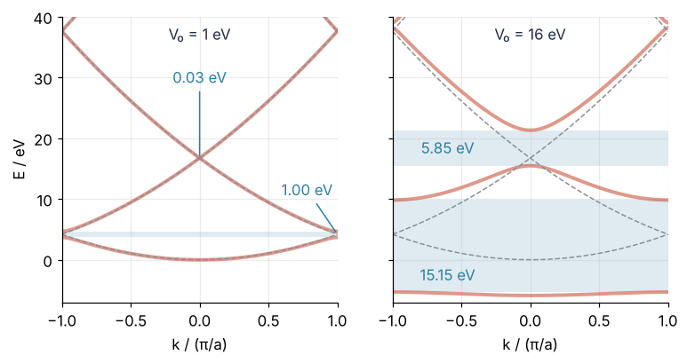
Energy bands for a weak (1 eV) and a strong (16 eV) cosine potential, energy in eV against k/(π/a). The first gap grows from 1.00 to 15.15 eV, and the lowest band flattens to 0.56 eV wide below zero.

At 16 eV the lowest band is 0.56 eV wide and sits below zero, an electron that barely moves between wells. The first gap is 15.15 eV, 5.3 % short of \(V_0\), and the second, which a cosine opens only at second order, has grown from 0.03 to 5.85 eV.

Pitfalls

Mixing SI and eV Å units. Every band comes out as a flat line between −0.99 and +0.99 eV, the same at every \(k\). The cause is \(\hbar^2/2m_e\) taken in J m², \(6.1 \times 10^{-39}\), while \(k\) is in 1/Å and \(V\) in eV: the kinetic diagonal is zero to machine precision, and the eigenvalues are those of the potential matrix alone. Pick one unit system, convert the constant into it as Setup does, and print the free energy at the zone boundary, 4.178 eV here, before you trust anything else.

Indexing the plane waves off by one. Shift the lookup in Step 2 by one and the matrix still builds, because a negative index wraps around in NumPy:

n = np.arange(-K, K + 1)
H_bad = Vm[n[:, None] - n[None, :] + 2 * K - 1] + np.diag(C * (np.pi / a + n * G0)**2)
print("Hermitian:", np.allclose(H_bad, H_bad.conj().T))
print("lowest two at k = pi/a:", np.round(np.linalg.eigvalsh(H_bad)[:2], 3), "eV")

Hermitian: False
lowest two at k = pi/a: [4.668 4.668] eV

The diagonal now carries \(V_{-1}\), the two lowest energies at the zone boundary land together at 4.668 eV, about 0.5 eV above the free 4.18 eV, and the first gap is gone. eigvalsh gives no warning, because it reads only one triangle of the matrix and assumes the other. Build n centered, as np.arange(-K, K + 1), and run np.allclose(H, H.conj().T) before every diagonalization.

Reading a gap off the k-grid. Step 4 uses 201 values of \(k\). Take 200 and the grid includes both zone boundaries but misses \(k = 0\), so the second gap read from the grid is 0.170 eV against the true 0.030 eV:

E200 = bands(1.0, np.linspace(-np.pi / a, np.pi / a, 200))
print(f"second gap from 200 k values: {E200[:, 2].min() - E200[:, 1].max():.3f} eV")

second gap from 200 k values: 0.170 eV

The bands are fine; the grid skips the point where the gap is narrowest. Compute band edges at the exact \(k = 0\) and \(k = \pi/a\), as Step 3 does, and use an odd number of \(k\) values for plots so that \(k = 0\) is on the grid.

Variations

Kronig-Penney square wells. Replace the cosine by a square well. Its Fourier components fall only as \(1/m\), so the bands converge slowly with \(N\) and you need many more plane waves and more samples per cell. The exact Kronig-Penney equation is the check.
Two atoms per cell. \(V(x) = V_0\cos(2\pi x/a) + W\cos(4\pi x/a)\): the second term opens the second gap at first order, \(2|V_2| = |W|\) by Step 4's rule. With \(V_0 = 1\) eV the matrix gives 0.429 eV for \(W = 0.4\) eV and 0.369 eV for \(W = -0.4\) eV, Step 3's second-order 0.03 eV added or taken away.
An exact reference. With a cosine the equation is Mathieu's. scipy.special.mathieu_a(1, q) and mathieu_b(1, q) with \(q = V_0/2E_\mathrm{f}\), times \(E_\mathrm{f}\), are the two band edges at the zone boundary (DLMF chapter 28). The matrix agrees with them to better than \(10^{-6}\) eV.
Two dimensions. \(G\) becomes a vector on the reciprocal lattice and \(k\) runs along a path between high-symmetry points. The matrix grows fast, which is where eigsh or a plane-wave electronic-structure code takes over.

Cheat sheet

x = np.arange(Ns) * a / Ns                                  # one cell, no endpoint
Vm = np.exp(-1j * np.outer(np.arange(-2*K, 2*K + 1), G0 * x)) @ V(x) / Ns   # V_m, m = -2K ... 2K
n = np.arange(-K, K + 1)                                    # centered plane-wave index
H = Vm[n[:, None] - n[None, :] + 2*K] + np.diag(C * (k + n * G0)**2)   # V_(n-n') off, kinetic on
assert np.allclose(H, H.conj().T)                           # before every eigh
E = np.linalg.eigvalsh(H)                                   # ascending; column j over k is band j
# band edges at exact k = 0 and k = pi/a; first-order gap n is about 2|V_n|
# grow 2K + 1 until the bands you plot stop moving; the top few are always wrong