python-control from the ground up: a car's suspension with a worn damper

The problem: a car body on a spring and a damper

One wheel of a car carries 250 kg of body on a spring of 16 kN/m, so the body bounces at \(\omega_0 = \sqrt{k/m} = 8\) rad/s, or 1.27 Hz. Put a 1 kN load in the trunk and the body ends up 6.25 cm lower. How it gets there depends on the damper. With a new one, rated at 2800 N s/m, the body dips 4.6 % past its final position and settles. With a worn one at 1000 N s/m it dips 44 % past, to 9.03 cm, and rings for almost two seconds. python-control, the Python library that speaks the language of control textbooks, models that wheel in a few lines and reads the state of the damper off its response.

The model is Newton's law for the body,

with \(m\) the mass, \(c\) the damper constant, \(k\) the spring constant, and \(x\) the deflection under the load, down positive. The one number that sums up the damper is the damping ratio \(\zeta = c/(2\sqrt{km})\), which is 0.25 for the worn damper and 0.7 for the new one. Below 1 the body rings after a bump; from 1 on it creeps back without overshoot.

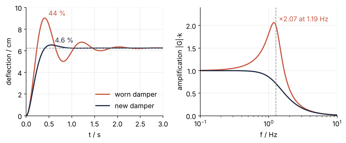
On the left is the response to the load, on the right how much a periodic push at each frequency is amplified. Both come from the same two models, through step_response and frequency_response, and both say the same thing about the worn damper.

Setup

import numpy as np
import matplotlib.pyplot as plt
import control

m = 250.0       # kg, body mass on one wheel
k = 16000.0     # N/m, spring
F0 = 1000.0     # N, load in the trunk
dampers = {"worn": 1000.0, "new": 2800.0}   # N s/m

plt.rcParams.update({
    "figure.figsize": (7, 3.6), "figure.dpi": 110,
    "axes.spines.top": False, "axes.spines.right": False,
    "axes.grid": True, "grid.alpha": 0.25,
    "font.size": 11, "lines.linewidth": 1.8,
})
INK, ACCENT, SECOND, MUTED = "#1f2a44", "#c8553d", "#2a7f9e", "#8a8f98"

# road for Step 4: ISO 8608 class C, explained there
rng = np.random.default_rng(8608)
v = 20.0                                   # m/s, 72 km/h
n = np.linspace(0.011, 2.83, 400)          # spatial frequencies, cycles/m
amp = np.sqrt(2 * 256e-6 * (n / 0.1) ** -2 * (n[1] - n[0]))
phase = rng.uniform(0, 2 * np.pi, n.size)
t_road = np.arange(0, 20, 0.01)            # s
road = (amp[:, None] * np.cos(2 * np.pi * n[:, None] * v * t_road + phase[:, None])).sum(axis=0)
road -= road[0]                            # start at zero height

omega0 = np.sqrt(k / m)
print(f"omega0 = {omega0:.2f} rad/s = {omega0 / (2 * np.pi):.2f} Hz")
for name, c in dampers.items():
    print(f"{name:4s} damper: zeta = {c / (2 * np.sqrt(k * m)):.2f}")
print(f"road: RMS height {1e3 * np.sqrt(np.mean(road**2)):.1f} mm")

omega0 = 8.00 rad/s = 1.27 Hz
worn damper: zeta = 0.25
new  damper: zeta = 0.70
road: RMS height 19.3 mm

The last lines draw a road profile for Step 4. Until then, treat road as given input: heights in meters, one every 0.01 s for 20 s.

Step 1: Write the suspension as a transfer function

A transfer function is the ratio of output to input for a linear system. With the body at rest at first, the Laplace transform turns every \(d/dt\) into a factor \(s\), so the differential equation turns into a ratio of polynomials:

The second form is the one textbooks use, and it shows where \(\omega_0\) and \(\zeta\) sit. In python-control you hand over the coefficients of numerator and denominator, highest power first:

G = {name: control.tf([1], [m, c, k], name=name) for name, c in dampers.items()}
print(G["worn"])
print(f"static deflection under F0: {control.dcgain(G['worn']) * F0:.4f} m")

<TransferFunction>: worn
Inputs (1): ['u[0]']
Outputs (1): ['y[0]']

              1
  --------------------------
  250 s^2 + 1000 s + 1.6e+04
static deflection under F0: 0.0625 m

The printout is the polynomial you wrote, \(250s^2 + 1000s + 1.6\cdot10^4\), in m/N. dcgain evaluates \(G\) at \(s = 0\), the response to a constant force, and gives the 6.25 cm from the opening. It is the same for both dampers, because a damper does nothing to a body at rest.

SciPy can do a step response too, with scipy.signal.lti and scipy.signal.step, and needs no extra install. Use it when a simulation is all you want. To read numbers off it, python-control carries what comes after, step_info, damp, Bode plots, feedback, in the vocabulary of control textbooks.

Step 2: Write the same model in state space

The other standard form is a set of first-order equations. Take the deflection \(x\) and the velocity \(v = \dot x\) as the state; then

control.ss takes the four matrices. python-control also converts a transfer function on its own, with tf2ss:

c = dampers["worn"]
A = np.array([[0, 1], [-k / m, -c / m]])
B = np.array([[0], [1 / m]])
C = np.array([[1, 0]])
D = np.array([[0]])
sys_worn = control.ss(A, B, C, D)

sys_conv = control.tf2ss(G["worn"])
print("A =", sys_conv.A.tolist(), "  C =", sys_conv.C.tolist())
print(control.ss2tf(sys_worn))

A = [[-4.0, -64.0], [1.0, 0.0]]   C = [[0.0, 0.004]]
<TransferFunction>: sys[2]
Inputs (1): ['u[0]']
Outputs (1): ['y[0]']

  -4.441e-16 s + 0.004
  --------------------
     s^2 + 4 s + 64

The converted matrices are not yours: its \(A\) has the \(-4\) and \(-64\) in the first row, and its \(C\) reads \(0.004 = 1/m\) off the second state. The state is a different pair of variables, and the system is the same. ss2tf of your own matrices gives back the denominator \(s^2 + 4s + 64\), which is \(G\) with top and bottom divided by \(m\), and a numerator term of order \(10^{-16}\) that is rounding, not physics. Compare models by their transfer functions or their responses, never by their matrices.

Step 3: Compute the step response and read the damping off the overshoot

step_response simulates the system after its input jumps from 0 to 1 at \(t = 0\). Multiplying a system by a number scales its input, so F0 * G is the response to a 1 kN step rather than 1 N. step_info measures the response for you:

t = np.linspace(0, 3, 601)
resp = {name: control.step_response(F0 * G[name], t) for name in dampers}

print("damper   peak / cm   at / s   overshoot   settled / s   final / cm")
info = {}
for name in dampers:
    info[name] = control.step_info(F0 * G[name])
    i = info[name]
    print(f"{name:6s} {100 * i['Peak']:9.2f} {i['PeakTime']:8.2f} {i['Overshoot']:9.1f} % "
          f"{i['SettlingTime']:11.2f} {100 * i['SteadyStateValue']:11.2f}")

damper   peak / cm   at / s   overshoot   settled / s   final / cm
worn        9.03     0.41      44.4 %        1.79        6.25
new         6.54     0.55       4.6 %        0.75        6.25

The response itself is in resp[name].time and resp[name].outputs, a plain array for one input and one output. The worn damper overshoots by 44.4 % and needs 1.79 s to stay within 2 % of its final value, which is what SettlingTime measures. The new one overshoots by 4.6 % and settles in 0.75 s.

The overshoot of a second-order system depends on \(\zeta\) alone, \(\mathrm{OS} = \exp(-\pi\zeta/\sqrt{1-\zeta^2})\). Solved for the damping ratio, that is

one line of code:

for name in dampers:
    OS = info[name]["Overshoot"] / 100
    print(f"{name:4s}: zeta from the overshoot = {-np.log(OS) / np.sqrt(np.pi**2 + np.log(OS)**2):.3f}")

worn: zeta from the overshoot = 0.250
new : zeta from the overshoot = 0.700

That is the damping read off a step response, 0.250 and 0.700. The same line works on a step response you measured on a test rig.

Step 4: Drive over a road with forced_response

On a road, heights point up. From here on \(x\) is the height of the body and \(r\) the height of the road under the wheel, both up positive and zero at rest. Spring and damper act on the difference:

With \(d/dt \to s\) again, the transfer function from road to body is \(X/R = (cs + k)/(ms^2 + cs + k)\).

The road from the Setup cell is generated, not measured. ISO 8608 classifies roads by their spectral density \(\Phi(n)\), the mean square height per unit of spatial frequency \(n\) in cycles/m. Long waves are large and short ones small: an average road, class C, has \(\Phi(n) = 256\cdot10^{-6}\,(n/0.1)^{-2}\) m³. The Setup cell adds 400 cosine waves, one per \(n\), each with a random phase and the amplitude \(\sqrt{2\Phi(n)\,\Delta n}\), so that its variance is \(\Phi(n)\,\Delta n\), the share of the spectrum in its band of width \(\Delta n\). Summing harmonics this way is the usual method in the vehicle literature; the standard itself only defines the spectrum and the classes. At 20 m/s a wave 16 m long passes at 1.25 Hz, right at the body's resonance.

forced_response simulates the response to any input you give it on an evenly spaced time grid:

body = {}
for name, c in dampers.items():
    Gr = control.tf([c, k], [m, c, k])
    body[name] = control.forced_response(Gr, T=t_road, U=road).outputs
    travel = body[name] - road
    print(f"{name:4s}: suspension travel RMS {1e3 * np.sqrt(np.mean(travel**2)):4.1f} mm, "
          f"largest {1e3 * np.abs(travel).max():4.1f} mm")

worn: suspension travel RMS 11.1 mm, largest 33.2 mm
new : suspension travel RMS  6.6 mm, largest 22.1 mm

Show code

Copy

window = (t_road >= 4) & (t_road <= 10)
colors = {"worn": ACCENT, "new": INK}
fig, (ax1, ax2) = plt.subplots(2, 1, sharex=True, figsize=(7, 4.4))
ax1.plot(t_road[window], 100 * road[window], color=SECOND, lw=1.2, label="road")
for name in dampers:
    ax1.plot(t_road[window], 100 * body[name][window], color=colors[name], label=f"body, {name} damper")
    travel = body[name] - road
    ax2.plot(t_road[window], 100 * travel[window], color=colors[name])
for x, name in [(0.01, "worn"), (0.42, "new")]:     # RMS over all 20 s, inside the panel above the data
    rms = 1e3 * np.sqrt(np.mean((body[name] - road)**2))
    ax2.text(x, 0.97, f"{name}: RMS {rms:.1f} mm", transform=ax2.transAxes, va="top", color=colors[name])
ax1.set(ylabel="height / cm", ylim=(-8.5, 4))
ax2.set(xlabel="t / s", ylabel="travel / cm", xlim=(4, 10), ylim=(-3.8, 3.8))
ax1.legend(frameon=False, ncols=3, loc="lower left", handlelength=1.5, columnspacing=1.2)
plt.show()

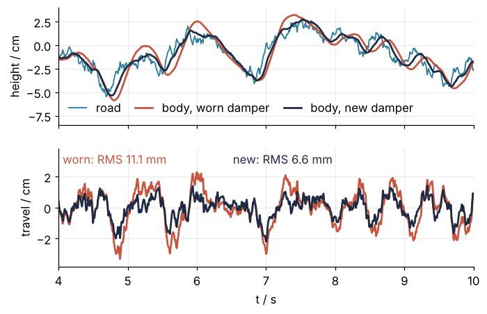
Both bodies follow the long waves of the road. Relative to the wheel, the worn damper swings 11.1 mm RMS and up to 33 mm, the new one 6.6 mm and up to 22 mm. A suspension has only so much travel, and the worn damper uses two thirds more of it.

Step 5: Find the poles and read the damping off them

The poles of \(G\) are the roots of its denominator, \(ms^2 + cs + k = 0\), which is the characteristic equation of the differential equation. Each pole \(p\) is a \(\lambda\) in a solution \(e^{\lambda t}\), so a complex pair \(p = -\sigma \pm i\omega_d\) means a decay \(e^{-\sigma t}\) times an oscillation at \(\omega_d\):

for name in dampers:
    print(f"{name:4s}: poles {np.round(control.poles(G[name]), 3)}")
control.damp(G["worn"]);

worn: poles [-2.+7.746j -2.-7.746j]
new : poles [-5.6+5.713j -5.6-5.713j]
    Eigenvalue (pole)       Damping     Frequency
        -2    +7.746j          0.25             8
        -2    -7.746j          0.25             8

The worn damper has its poles at \(-2 \pm 7.746i\), the new one at \(-5.6 \pm 5.713i\). Both pairs lie on a circle of radius \(|p| = \omega_0 = 8\) rad/s, and the damping ratio is the share of the real part, \(\zeta = -\mathrm{Re}\,p/|p|\): 2/8 = 0.25 and 5.6/8 = 0.7, as damp prints. The real part also sets how fast the ringing dies. The envelope \(e^{-\sigma t}\) falls to 2 % after \(\ln 50/\sigma \approx 4/\sigma\), which is 2.0 s for the worn damper and 0.71 s for the new one, against 1.79 s and 0.75 s from step_info: a rule of thumb, good to about 10 %.

The poles are also the eigenvalues of \(A\), which is why the two different matrices of Step 2 describe one system (the eigenvalue tutorial has more on these):

print(np.round(np.linalg.eigvals(A), 3), np.round(np.linalg.eigvals(sys_conv.A), 3))

[-2.+7.746j -2.-7.746j] [-2.+7.746j -2.-7.746j]

Both matrices give \(-2 \pm 7.746i\), the poles of the worn damper.

Step 6: Read the resonance off the Bode plot

Push the body with a force \(F_0 \sin\omega t\) and, once the start-up has died away with Step 5's \(e^{-\sigma t}\), it moves as a sine of the same frequency. The amplitude is scaled by \(|G(i\omega)|\) and the motion lags by the angle of the complex number \(G(i\omega)\) in the plane. You get \(G(i\omega)\) by putting \(s = i\omega\), since the derivative of \(e^{i\omega t}\) is \(i\omega\) times itself, which is the rule of Step 1 again. A Bode plot draws the magnitude and the phase against \(\omega\):

Copy

omega = np.logspace(-1, 2, 2000)    # rad/s
cp = control.bode_plot(G["worn"], omega, color=ACCENT, label="worn", title=False, legend_loc=False,
                       rcParams=plt.rcParams)  # the font sizes of the setup cell, not python-control's smaller ones
control.bode_plot(G["new"], omega, color=INK, label="new", ax=cp.axes, title=False, legend_loc=False)
ax_mag, ax_phase = cp.axes[:, 0]
for ax in (ax_mag, ax_phase):
    ax.grid(False, which="minor")                  # bode_plot draws minor grid lines; keep the major ones
    ax.axvline(omega0, color=MUTED, ls="--", lw=1)  # natural frequency, 8 rad/s
ax_mag.set(ylabel="|G| / (m/N)")
ax_phase.set(xlabel="ω / (rad/s)", ylabel="phase / degrees")
ax_mag.legend(frameon=False)
plt.show()

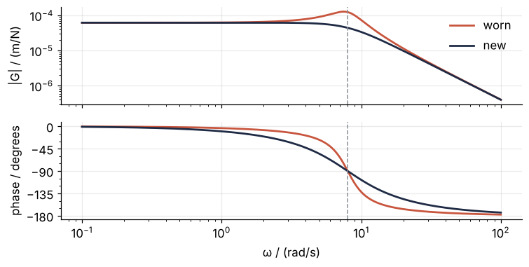
Below \(\omega_0\) both magnitudes sit at \(1/k = 6.25\cdot10^{-5}\) m/N, the static deflection per newton; above it they fall and merge. Only the worn damper has a peak, just below \(\omega_0\), and both phases pass \(-90°\) at 8 rad/s, whatever the damping. For numbers, frequency_response returns the same curve as arrays; multiplied by \(k\), the magnitude is the amplification over the static deflection. For a second-order system the peak has the height \(M_r = 1/(2\zeta\sqrt{1-\zeta^2})\), which solved for the damping ratio is

gain = {name: control.frequency_response(G[name], omega).magnitude * k for name in dampers}
for name in dampers:
    i = gain[name].argmax()
    print(f"{name:4s}: largest amplification {gain[name][i]:.4f} at {omega[i]:.2f} rad/s = {omega[i] / (2 * np.pi):.2f} Hz")

Mr = gain["worn"].max()
print(f"worn: zeta from the peak = {np.sqrt((1 - np.sqrt(1 - 1 / Mr**2)) / 2):.3f}")

worn: largest amplification 2.0656 at 7.49 rad/s = 1.19 Hz
new : largest amplification 1.0002 at 1.13 rad/s = 0.18 Hz
worn: zeta from the peak = 0.250

The worn damper amplifies by 2.07 at 1.19 Hz, and its peak gives 0.250 again. The new one reaches 1.0002, a bump of two parts in ten thousand at 0.18 Hz: at \(\zeta = 0.7\) the curve is about as flat as a spring and a damper can make it.

bode_plot draws on its own axes, so the figure from the opening puts the step responses and the amplification side by side by hand:

Copy

f = omega / (2 * np.pi)
colors = {"worn": ACCENT, "new": INK}
fig, (ax1, ax2) = plt.subplots(1, 2, figsize=(8, 3.4))
for name in dampers:
    ax1.plot(resp[name].time, 100 * resp[name].outputs, color=colors[name], label=f"{name} damper")
    ax2.semilogx(f, gain[name], color=colors[name])
    ax1.annotate(f"{info[name]['Overshoot']:.2g} %", (info[name]["PeakTime"], 100 * info[name]["Peak"]),
                 xytext=(6, 4), textcoords="offset points", color=colors[name])
ax1.axhline(100 * F0 / k, color=MUTED, ls="--", lw=1)
ax1.set(xlabel="t / s", ylabel="deflection / cm", xlim=(0, 3), ylim=(0, 10))
ax1.legend(frameon=False, loc="lower right")
i = gain["worn"].argmax()
ax2.axvline(omega0 / (2 * np.pi), color=MUTED, ls="--", lw=1)
ax2.annotate(f"×{gain['worn'][i]:.2f} at {f[i]:.2f} Hz", (f[i], gain["worn"][i]),
             xytext=(8, 2), textcoords="offset points", color=ACCENT)
ax2.set(xlabel="f / Hz", ylabel="amplification |G|·k", xlim=(0.1, 10), ylim=(0, 2.4))
fig.tight_layout()
plt.show()

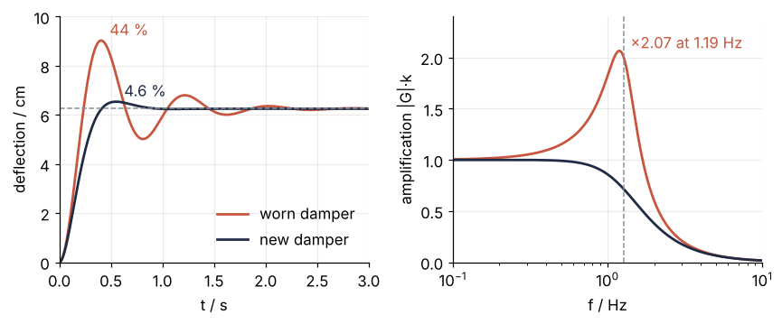
The dashed lines mark the static deflection, 6.25 cm, and the natural frequency, 1.27 Hz. The 44 % overshoot on the left and the factor 2 on the right are the same weak damping, seen once in time and once in frequency.

Pitfalls

Hertz where python-control wants rad/s. You ask for the response at the body's resonance, 1.27 Hz, and get an amplification of 1.02 instead of about 2:

print(control.frequency_response(G["worn"], [1.27]).magnitude * k,     # 1.27 read as rad/s
      control.frequency_response(G["worn"], [8.0]).magnitude * k)      # 8 rad/s = 1.27 Hz

[1.02246903] [2.]

The frequencies you pass to frequency_response and bode_plot are angular, in rad/s. bode_plot(..., Hz=True) only relabels the axis in Hz. Combined with omega_limits=[0.1, 10], version 0.10.2 sets the axis to 0.1 to 10 Hz but computes the curve from 0.1 to 10 rad/s, so it stops at 1.59 Hz. Multiply by \(2\pi\) on the way in and divide on the way out.

Measured inputs on an uneven clock. With logged data whose timestamps jitter, forced_response stops with ValueError: Parameter `T`: time values must be equally spaced. The solver turns the system into a discrete one with a single fixed step, so it needs a single step in the data. Put the input on a regular grid first, with np.interp(np.arange(t0, t1, dt), t_logged, u_logged).

Old code that calls control.pole. Code from older answers and lecture notes fails with AttributeError: module 'control' has no attribute 'pole'. The singular names pole and zero were deprecated and are gone in version 0.10. Use control.poles and control.zeros, and check control.__version__ against the documentation you are reading.

Variations

• A curb instead of a road. control.step_response(Gr) with the road transfer function of Step 4. The root of the numerator, \(s = -k/c\), adds overshoot: 50.6 % with the worn damper and 21.0 % with the new one, so the inversion of Step 3 does not apply. control.zeros(Gr) finds that root.
• Comfort against grip. Take the body's acceleration as the output and the picture turns: above \(\sqrt2\,\omega_0\) a harder damper passes more of the road to the body. That is why comfort-tuned suspensions sit near \(\zeta = 0.3\) to 0.4, not 0.7.
• A quarter car with its wheel. Add the wheel, about 40 kg, on a tire of about 200 kN/m. Four states and two resonances, the body near 1.2 Hz and wheel hop near 12 Hz; control.ss, poles, and bode_plot carry over unchanged, and this is where state space pays off.
• Close a loop. An active suspension measures the body's motion and pushes back. control.feedback(G, K) closes the loop around a controller K.

Cheat sheet

sys = control.tf(num, den)                  # coefficients, highest power of s first
sys = control.ss(A, B, C, D)                # state space; tf2ss / ss2tf convert
resp = control.step_response(sys, t)        # resp.time, resp.outputs
info = control.step_info(sys)               # "Peak", "PeakTime", "Overshoot" in %, "SettlingTime" (2 %)
resp = control.forced_response(sys, T=t, U=u)   # any input; t evenly spaced
control.poles(sys); control.damp(sys)       # zeta = -Re(p) / |p|
control.bode_plot(sys, omega)               # omega array in rad/s, even with Hz=True
mag = control.frequency_response(sys, omega).magnitude
control.dcgain(sys)                         # response to a constant input

Further reading

• The python-control documentation, with the function reference and the chapters on time and frequency responses.
• Åström and Murray, Feedback Systems, 2nd edition, free online; chapter 6 covers step responses and chapter 9 transfer functions and Bode plots. Gillespie, Fundamentals of Vehicle Dynamics, for the quarter-car model and road roughness.
• Related tutorials on this site: solve_ivp from the ground up: the pendulum beyond small angles, Eigenvalues with numpy.linalg: normal modes of coupled oscillators, The Kalman filter: a battery's charge from a drifting current and noisy voltage, Filtering with scipy.signal: mains hum and noise out of an ECG, Grid frequency after a power plant trips: the nadir with half the inertia. Planned: The same suspension in Julia with ControlSystems.jl.
• Download the notebook. It was executed with the library versions in the header.