System identification: a DC motor's model from its voltage and speed
Afterwards you can explain how an ARX model is fitted by least squares, why the input must excite every frequency that matters, and how to validate the model.
- Field
- Engineering, Physics
- Prerequisites
- Least squares: what a fit minimizes, and why the residuals are squared, The Fourier transform: asking a signal how much of each frequency it contains, python-control from the ground up: a car's suspension with a worn damper
- Libraries
control 0.10.2matplotlib 3.11.2numpy 2.4.3scipy 1.18.1
py-system-identification.ipynb, executed with the versions above. The download needs a free account
Run it yourself. In a terminal, this installs exactly the versions above:
pip install numpy==2.4.3 scipy==1.18.1 control==0.10.2 matplotlib==3.11.2 jupyterlabThe question
A small DC motor sits on a bench. A digital drive sets its voltage 100 times a second, and a sensor logs its speed at the same rate, with a noise of 0.02 rad/s. Ten seconds give 1000 samples of voltage and 1000 of speed, and nobody hands you the motor's transfer function. Getting a model out of such records is called system identification. Here are two experiments on the same motor: on the left a voltage step from 0 to 6 V after 1 s, on the right a voltage that switches between 3 V and 9 V, with a coin flip every 50 ms deciding which.
Show code
import numpy as np
import matplotlib.pyplot as plt
import control
from scipy.signal import lfilter

plt.rcParams.update({
    "figure.figsize": (7, 3.6), "figure.dpi": 110,
    "axes.spines.top": False, "axes.spines.right": False,
    "axes.grid": True, "grid.alpha": 0.25,
    "font.size": 11, "lines.linewidth": 1.8,
})
INK, ACCENT, SECOND, MUTED = "#1f2a44", "#c8553d", "#2a7f9e", "#8a8f98"

# The lab. The motor is simulated, so that every fitted number can be checked against the truth.
# Pretend you have not seen this cell.
dt, N = 0.01, 1000                                  # 100 samples per second, 10 s
t = np.arange(N) * dt
K, tau_m, tau_e = 20.0, 0.25, 0.05                  # rad/s per V, s, s
# tau_e = 0.05 s is illustrative: in real small motors it is a few ms or less, too fast to see at 100 Hz
motor = control.tf(K, np.polymul([tau_m, 1], [tau_e, 1]))
motor_d = control.c2d(motor, dt, "zoh")             # the drive holds each voltage for one sample
den_true = np.ravel(motor_d.den[0][0])
num_true = np.r_[0, np.ravel(motor_d.num[0][0])]    # leading zero: the speed answers one sample later

rng = np.random.default_rng(126)
u_step = np.where(t >= 1.0, 6.0, 0.0)                                 # V
u_rand = np.repeat(rng.choice([3.0, 9.0], N // 5), 5)                 # a new coin flip every 50 ms
levels, holds = rng.uniform(2, 10, 200), rng.integers(5, 31, 200)     # 2 to 10 V, held 50 to 300 ms
u_val = np.repeat(levels, holds)[:N]

sigma = 0.02                                                          # rad/s, the speed sensor's noise
def measure(u, noise=sigma, gen=rng):
    return lfilter(num_true, den_true, u) + noise * gen.standard_normal(u.size)

y_step, y_rand, y_val = measure(u_step), measure(u_rand), measure(u_val)
p_true = np.sort(np.roots(den_true))[::-1]
print(f"true motor: gain {K:.0f} rad/s per V, decay factors per sample {p_true[0]:.4f} and {p_true[1]:.4f}")

fig, axes = plt.subplots(2, 2, figsize=(8, 4.4), sharex=True, sharey="row")
for col, (u, y, color) in enumerate([(u_step, y_step, SECOND), (u_rand, y_rand, ACCENT)]):
    axes[0, col].plot(t, u, color=color, lw=1.2)
    axes[1, col].plot(t, y, color=INK, lw=1.2)
    axes[1, col].set_xlabel("t / s")
    axes[0, col].text(0.02, 0.97, ["step", "random binary"][col], color=color,
                      transform=axes[0, col].transAxes, va="top")
axes[0, 0].set(ylabel="voltage / V", xlim=(0, 10), ylim=(-0.5, 12.5), yticks=[0, 3, 6, 9])
axes[1, 0].set(ylabel="speed / rad/s")
fig.align_ylabels(axes[:, 0])
plt.show()
true motor: gain 20 rad/s per V, decay factors per sample 0.9608 and 0.8187
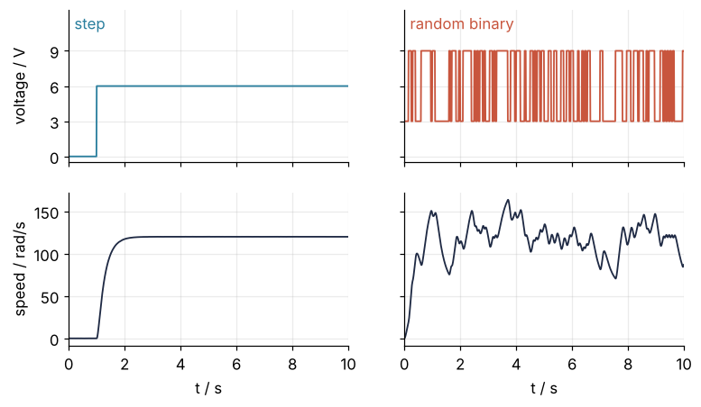
Two things are obvious. The step response settles at 120 rad/s, so the motor gives 20 rad/s per volt, and it gets there within about a second. The random record looks like noise on top of noise: the speed swings up and down with every run of coin flips and never settles anywhere.
Less obvious is which record tells you the motor's model. Both come from the same motor, and the step looks like the cleaner experiment. And since any model with enough parameters reproduces the record it was fitted to, how would you know a good one when you see it? The fitting itself is the easy part, a difference equation and the least squares you already know. What decides the answer is the input you choose and the check you apply afterwards.
The idea: every sample is an equation
A linear motor sampled every \(\Delta t = 0.01\) s obeys a difference equation. Each new speed \(y[k]\) is a weighted sum of the two speeds before it and the two voltages \(u\) before it:
Two past values of each, because the motor has two time constants, a mechanical one for the rotor and an electrical one for the winding. Read this way, every sample of the record is one linear equation for the four unknown weights \(a_1, a_2, b_1, b_2\). Ten seconds supply 998 of them, the first two samples having no past, and least squares finds the four weights that miss them least. The model is called ARX, autoregressive with an exogenous input: the speed is regressed on its own past and on the voltage.
Four weights are not what an engineer reads off a motor, so translate them. When the speed is steady, all the \(y\) are equal and all the \(u\) are equal, and the equation becomes \((1 + a_1 + a_2)\,y = (b_1 + b_2)\,u\): the gain is \((b_1 + b_2)/(1 + a_1 + a_2)\). With the voltage off, try a speed that decays geometrically, \(y[k] = p^k\). Put it into the equation, divide by \(p^{k-2}\), and what is left is \(p^2 + a_1 p + a_2 = 0\). So there are two decay factors \(p_1\) and \(p_2\), the roots of that quadratic, and multiplying out \((p - p_1)(p - p_2)\) shows \(a_1 = -(p_1 + p_2)\) and \(a_2 = p_1 p_2\). A decay \(p^k\) is the same as \(e^{-k\Delta t/\tau}\), so each root is a time constant, \(\tau = -\Delta t/\ln p\). The motor here has decay factors 0.9608 and 0.8187 per sample, which give 0.25 s and 0.05 s. The electrical 0.05 s is chosen larger than in most small motors, where it is a few milliseconds or less, so that both time constants show at 100 samples a second.
Here are three of the step record's 998 equations, each a row of the matrix least squares works on, with the speed it must reproduce:
Show code
def regressor(u, y, na=2, nb=2):
    """One row per sample k: (-y[k-1], ..., -y[k-na], u[k-1], ..., u[k-nb]), and the targets y[k]."""
    n = max(na, nb)
    Phi = np.column_stack([-y[n - i:y.size - i] for i in range(1, na + 1)]
                          + [u[n - i:u.size - i] for i in range(1, nb + 1)])
    return Phi, y[n:]

Phi_step, Y_step = regressor(u_step, y_step)
print("   t      -y[k-1]   -y[k-2]   u[k-1]  u[k-2]   |   y[k]")
for tk in [0.5, 1.05, 5.0]:
    i = round(tk / dt) - 2                          # row i belongs to sample k = i + 2
    print(f"{tk:5.2f} s " + "".join(f"{v:9.3f}" for v in Phi_step[i]) + f"   | {Y_step[i]:8.3f}")
   t      -y[k-1]   -y[k-2]   u[k-1]  u[k-2]   |   y[k]
 0.50 s     0.007    0.007    0.000    0.000   |   -0.006
 1.05 s    -5.671   -3.441    6.000    6.000   |    8.192
 5.00 s  -119.976 -120.000    6.000    6.000   |  119.985
At 0.5 s, before the step, the row is sensor noise and says nothing. At 1.05 s the motor is accelerating, and the row carries how it does so. At 5 s the motor has settled, and the row says \(120\,(1 + a_1 + a_2) = 6\,(b_1 + b_2)\), which is the gain equation from above, 20 rad/s per V. Every row after about 2 s says the same. The step record is mostly one equation repeated 800 times.
To see what that does to the fit, map the misfit over the two time constants. Pick a pair of time constants; that fixes the two roots and so \(a_1\) and \(a_2\). Least squares then picks the best \(b_1\) and \(b_2\) for that pair, and the misfit left over is the height of the map at that point. The contours are drawn at 1.1, 1.5, 3, 10, 30, and 100 times the lowest misfit:
Show code
def misfit_map(u, y, tau_fast, tau_slow):
    """Least-squares misfit for every pair of time constants, with b1 and b2 fitted for each pair."""
    Phi, Y = regressor(u, y)
    Q, _ = np.linalg.qr(Phi[:, 2:])                                  # the two voltage columns
    W = np.column_stack([Y, -Phi[:, 0], -Phi[:, 1]])                  # y[k], y[k-1], y[k-2]
    R = W - Q @ (Q.T @ W)                                             # what b1, b2 cannot explain
    M = R.T @ R
    p1, p2 = np.exp(-dt / tau_slow), np.exp(-dt / tau_fast)
    v = np.stack([np.ones_like(p1), -(p1 + p2), p1 * p2])            # (1, a1, a2) for every pair
    return np.einsum("i...,ij,j...->...", v, M, v)

te, tm = np.meshgrid(np.geomspace(0.01, 0.15, 150), np.geomspace(0.12, 0.6, 150))
fig, axes = plt.subplots(1, 2, figsize=(8, 3.6), sharey=True)
for ax, (u, y, color, name) in zip(axes, [(u_step, y_step, SECOND, "step"), (u_rand, y_rand, ACCENT, "random binary")]):
    S = misfit_map(u, y, te, tm)
    ax.contour(te, tm, S / S.min(), levels=[1.1, 1.5, 3, 10, 30, 100], colors=color, linewidths=1)
    j = np.unravel_index(S.argmin(), S.shape)
    inside = te[S < 1.1 * S.min()]                                   # within 10 % of the best misfit
    print(f"{name:14s} best fast time constant {te[j]:.3f} s; within 10 % of the best misfit: "
          f"{inside.min():.3f} to {inside.max():.3f} s")
    ax.plot(tau_e, tau_m, "x", color=MUTED, ms=9, mew=2)
    ax.plot(te[j], tm[j], "o", color=color, ms=6)                    # on top: on the right it sits on the cross
    ax.set(xscale="log", yscale="log", xlabel="fast time constant / s",
           xticks=[0.01, 0.02, 0.05, 0.1], xticklabels=["0.01", "0.02", "0.05", "0.1"],
           yticks=[0.15, 0.25, 0.4, 0.6], yticklabels=["0.15", "0.25", "0.4", "0.6"])
    ax.minorticks_off()
    ax.text(0.98, 0.97, name, color=color, transform=ax.transAxes, ha="right", va="top",
            bbox=dict(fc="white", ec="none", pad=1))
    if name == "step":                                               # name the two marks once
        ax.annotate("truth", (tau_e, tau_m), xytext=(0.09, 0.46), color=MUTED, ha="center",
                    arrowprops=dict(arrowstyle="-", color=MUTED, lw=0.8, shrinkB=6))
        ax.annotate("best fit", (te[j], tm[j]), xytext=(0.0172, 0.46), color=color, ha="center",
                    arrowprops=dict(arrowstyle="-", color=color, lw=0.8, shrinkB=5))
axes[0].set_ylabel("slow time constant / s")
plt.show()
step           best fast time constant 0.040 s; within 10 % of the best misfit: 0.028 to 0.069 s
random binary  best fast time constant 0.049 s; within 10 % of the best misfit: 0.046 to 0.054 s
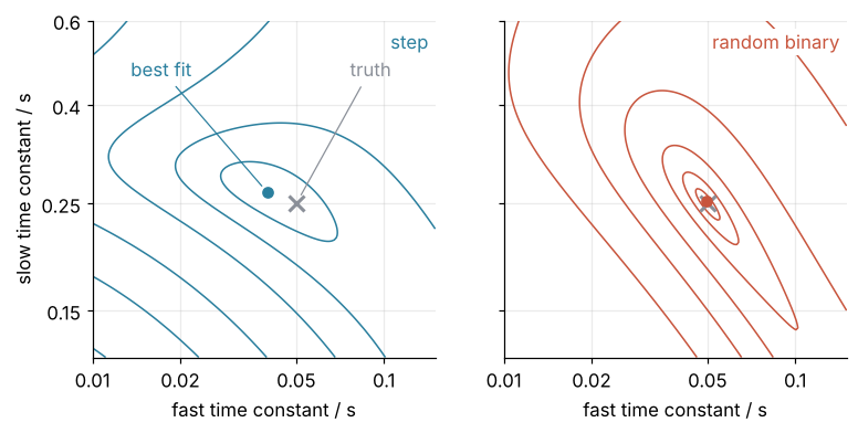
On the random record the misfit is a tight bowl around the truth: every fast time constant from 0.046 to 0.054 s comes within 10 % of the best fit. On the step record the same 10 % admits anything from 0.028 to 0.069 s, a valley five times wider, and its lowest point sits at 0.040 s. Along that valley the data barely care what the fast time constant is, so the sensor noise decides.
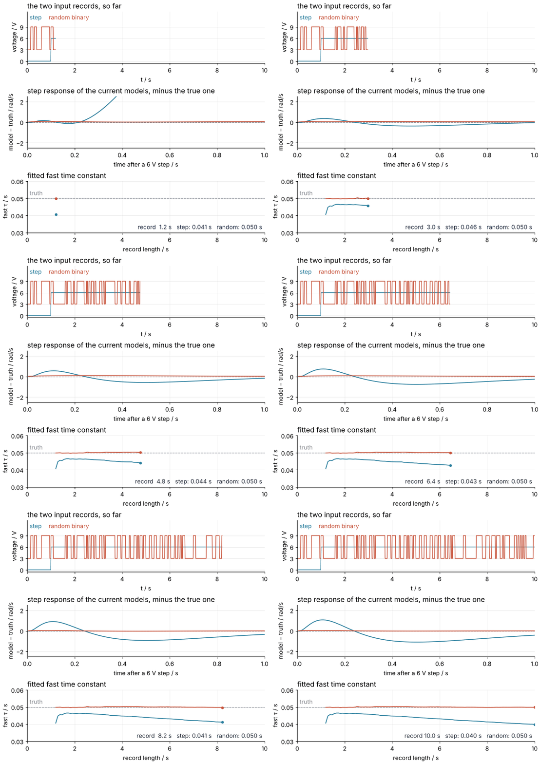
A longer record does not help. The animation refits both models as the record grows from 1.2 s to 10 s; watch the bottom panel.
Show code
"""ARX fits on a growing record: a step and a random binary input, same motor.

Renders ../../assets/arx-growing-record.gif. The data are those of the tutorial
py-system-identification: same motor, same seed, same order of draws. Run it from any directory:

    python scene.py
"""
from pathlib import Path

import numpy as np
import matplotlib.pyplot as plt
import control
from matplotlib.animation import FuncAnimation, PillowWriter
from PIL import Image
from scipy.signal import lfilter

OUT = Path(__file__).resolve().parents[2] / "assets" / "arx-growing-record.gif"
INK, ACCENT, SECOND, MUTED = "#1f2a44", "#c8553d", "#2a7f9e", "#8a8f98"
plt.rcParams.update({"axes.spines.top": False, "axes.spines.right": False,
                     "axes.grid": True, "grid.alpha": 0.25, "font.size": 11})

# ---- data: the motor and the two experiments of the tutorial
dt, N = 0.01, 1000
t = np.arange(N) * dt
tau_m, tau_e = 0.25, 0.05
motor_d = control.c2d(control.tf(20.0, np.polymul([tau_m, 1], [tau_e, 1])), dt, "zoh")
den_true = np.ravel(motor_d.den[0][0])
num_true = np.r_[0, np.ravel(motor_d.num[0][0])]
rng = np.random.default_rng(126)
u_step = np.where(t >= 1.0, 6.0, 0.0)
u_rand = np.repeat(rng.choice([3.0, 9.0], N // 5), 5)
rng.uniform(2, 10, 200), rng.integers(5, 31, 200)                   # the validation input: drawn, not used here
y_step = lfilter(num_true, den_true, u_step) + 0.02 * rng.standard_normal(N)
y_rand = lfilter(num_true, den_true, u_rand) + 0.02 * rng.standard_normal(N)

def arx(u, y):
    """Second-order ARX by least squares: A = (1, a1, a2), B = (0, b1, b2)."""
    Phi = np.column_stack([-y[1:-1], -y[:-2], u[1:-1], u[:-2]])
    theta = np.linalg.lstsq(Phi, y[2:], rcond=None)[0]
    return np.r_[1, theta[:2]], np.r_[0, theta[2:]]

def fast_tau(a):
    return np.min(-dt / np.log(np.abs(np.roots(a))))

lengths = np.linspace(1.2, 10, 100)                                 # s, one record length per frame
fits = {name: [arx(u[:round(L / dt)], y[:round(L / dt)]) for L in lengths]
        for name, u, y in [("step", u_step, y_step), ("random", u_rand, y_rand)]}
taus = {name: np.array([fast_tau(a) for a, b in fits[name]]) for name in fits}
t_resp = t[t <= 1.0]
volts = np.full(t_resp.size, 6.0)                                   # a 6 V step, as in the experiment
truth_resp = lfilter(num_true, den_true, volts)
resp_err = {name: np.array([lfilter(b, a, volts) - truth_resp for a, b in fits[name]]) for name in fits}
for name in taus:
    print(f"{name:6s} model, fast time constant at {lengths[0]:.1f} s: {taus[name][0]:.4f} s, "
          f"at 2 s: {np.interp(2, lengths, taus[name]):.4f} s, at 10 s: {taus[name][-1]:.4f} s; "
          f"step-response error at 10 s: {np.abs(resp_err[name][-1]).max():.2f} rad/s")

# ---- figure, drawn once
fig, (ax1, ax2, ax3) = plt.subplots(3, 1, figsize=(7, 6.6), dpi=80, layout="constrained")
(rec_step,) = ax1.plot([], [], color=SECOND, lw=1.2)
(rec_rand,) = ax1.plot([], [], color=ACCENT, lw=1.2)
ax1.text(0.01, 0.96, "step", color=SECOND, transform=ax1.transAxes, va="top")      # names the colors once
ax1.text(0.09, 0.96, "random binary", color=ACCENT, transform=ax1.transAxes, va="top")
ax1.set(xlim=(0, 10), ylim=(-0.5, 13), yticks=[0, 3, 6, 9], xlabel="t / s", ylabel="voltage / V")
ax2.axhline(0, color=MUTED, ls="--", lw=1)                          # the truth: no error
(resp_step,) = ax2.plot([], [], color=SECOND)
(resp_rand,) = ax2.plot([], [], color=ACCENT)
ax2.set(xlim=(0, 1.0), ylim=(-2.5, 2.5), xlabel="time after a 6 V step / s", ylabel="model − truth / rad/s")
ax3.axhline(tau_e, color=MUTED, ls="--", lw=1)
ax3.text(0.1, tau_e + 0.001, "truth", color=MUTED, va="bottom")
(tau_step,) = ax3.plot([], [], color=SECOND, marker="o", ms=4, markevery=[-1])   # a dot on the newest fit
(tau_rand,) = ax3.plot([], [], color=ACCENT, marker="o", ms=4, markevery=[-1])
label = ax3.text(0.99, 0.04, "", transform=ax3.transAxes, ha="right", va="bottom", color=INK)
ax3.set(xlim=(0, 10), ylim=(0.03, 0.06), xlabel="record length / s", ylabel="fast τ / s")
ax1.set_title("the two input records, so far", loc="left")
ax2.set_title("step response of the current models, minus the true one", loc="left")
ax3.set_title("fitted fast time constant", loc="left")

# ---- one frame: everything follows from the frame index
def update(i):
    n = round(lengths[i] / dt)
    rec_step.set_data(t[:n], u_step[:n])
    rec_rand.set_data(t[:n], u_rand[:n])
    resp_step.set_data(t_resp, resp_err["step"][i])
    resp_rand.set_data(t_resp, resp_err["random"][i])
    tau_step.set_data(lengths[:i + 1], taus["step"][:i + 1])
    tau_rand.set_data(lengths[:i + 1], taus["random"][:i + 1])
    label.set_text(f"record {lengths[i]:4.1f} s   step: {taus['step'][i]:.3f} s   "
                   f"random: {taus['random'][i]:.3f} s")

# ---- render, and read back what was written
OUT.parent.mkdir(exist_ok=True)
FuncAnimation(fig, update, frames=range(lengths.size)).save(OUT, writer=PillowWriter(fps=12))
plt.close(fig)
with Image.open(OUT) as im:
    delay = im.info["duration"]
    print(f"{OUT.name}: {im.width} x {im.height} px, {im.n_frames} frames at {delay} ms, "
          f"{im.n_frames * delay / 1000:.1f} s, {OUT.stat().st_size / 1024:,.0f} kB")
The random-input model has the fast time constant at 0.050 s after 1.2 s and keeps it. The step model reaches 0.046 s at 2 s, while the transient is still a sizable part of the record, and then drifts away to 0.040 s as each new second adds 100 more copies of the gain equation. At 10 s its response to a 6 V step is off by up to 1.10 rad/s, against 0.04 rad/s for the random-input model.
Why a step tells you the gain and little else
The reason is in what the two inputs contain, frequency by frequency, read the way the Fourier transform reads a signal. Each time constant \(\tau\) has a corner frequency \(1/(2\pi\tau)\): below it that part of the motor follows the voltage, above it a wiggle of the voltage comes out smaller and later. The motor's corners are at 0.64 Hz and 3.18 Hz. A fit learns what the motor does only at frequencies the input contains. One number per input says how much it contains up there, its power share above a frequency: square the spectrum, add up the squares above that frequency, and divide by the sum of all of them.
Show code
f = np.fft.rfftfreq(N, dt)
fig, ax = plt.subplots()
for u, color, name in [(u_step, SECOND, "step"), (u_rand, ACCENT, "random binary")]:
    X = np.fft.rfft(u - u.mean())
    power = np.abs(X) ** 2
    share = {fc: power[f > fc].sum() / power.sum() for fc in (0.5, 2.0)}
    print(f"{name:14s} power above 0.5 Hz: {share[0.5]:5.1%}   above 2 Hz: {share[2.0]:5.1%}")
    amp = 2 * np.abs(X[1:]) / N
    keep = amp > 1e-9                       # the step's exact zeros, at whole hertz, have no place on a log axis
    ax.plot(f[1:][keep], amp[keep], color=color, lw=1.2)
for tau in (tau_m, tau_e):
    fc = 1 / (2 * np.pi * tau)
    ax.axvline(fc, color=MUTED, ls="--", lw=1)
    ax.text(fc * 1.06, 2, f"{fc:.2f} Hz", color=MUTED)
ax.set(xscale="log", yscale="log", xlim=(0.1, 50), ylim=(1e-3, 5),
       xlabel="frequency / Hz", ylabel="amplitude / V")
ax.text(1.0, 0.02, "step", color=SECOND)              # below the step's lobes
ax.text(10, 1.2, "random binary", color=ACCENT)       # above the random input's flat top
plt.show()
step           power above 0.5 Hz: 20.9%   above 2 Hz:  5.6%
random binary  power above 0.5 Hz: 93.6%   above 2 Hz: 74.1%
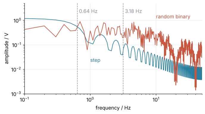
The step's spectrum is the spectrum of a single jump: it falls steadily from zero frequency, and both corners of the motor lie on its falling flank. Only 20.9 % of its power lies above 0.5 Hz and 5.6 % above 2 Hz, against 93.6 % and 74.1 % for the random input. At zero frequency the step tells you the gain, with 800 samples to spare. Above a hertz it says little, and the fast time constant, whose corner is at 3.18 Hz, is left to the noise.
The random input's spectrum stays flat that far because of its 50 ms clock. A signal that holds each value for 50 ms has its first null at \(1/(50\text{ ms}) = 20\) Hz, the dip at the right of the figure. A coin flip every half second would put that null at 2 Hz, below the fast corner, and starve the fast time constant almost as badly as the step does.
Formalization
The general ARX model of orders \(n_a\) and \(n_b\) is the same equation with more terms,
where \(e[k]\) is whatever the equation misses: noise, and anything the model leaves out. Control texts shorten it to \(A(q)\,y = B(q)\,u + e\), with \(q^{-1}\) the shift back by one sample, \(q^{-1}y[k] = y[k-1]\), so that \(A(q) = 1 + a_1 q^{-1} + \dots\) and \(B(q) = b_1 q^{-1} + \dots\). Each sample gives one row \(\varphi_k = (-y[k-1], \dots, -y[k-n_a],\ u[k-1], \dots, u[k-n_b])\). The rows stack into a matrix \(\Phi\), the speeds into a vector \(Y\), and the weights \(\theta = (a_1, \dots, b_{n_b})\) solve \(\Phi\theta \approx Y\) in the least-squares sense, one call to np.linalg.lstsq.
For any order, the gain is \(B(1)/A(1)\), and each root \(p\) of \(z^{n_a} + a_1 z^{n_a-1} + \dots + a_{n_a}\) gives \(\tau = -\Delta t/\ln p\). To get the transfer function, write the model as \(y = \big(B(q)/A(q)\big)\,u\), multiply top and bottom by \(q^2\) to clear the negative powers, and rename \(q\) to \(z\):
Here \(z\) plays the role \(s\) plays in python-control from the ground up: the roots of the denominator are the poles, here the decay factors \(p_1\) and \(p_2\). Starting \(B\) at \(u[k-1]\) assumes the speed reacts one sample after the voltage. With a dead time of \(d\) samples it starts at \(u[k-d]\), and \(d\) is chosen like the order.
Persistent excitation. An input that carries power at enough distinct frequencies to pin down every weight is called persistently exciting. After its transient a step carries one frequency, zero, and pins down one number, the gain. The condition number of \(\Phi\) measures the damage. It says how many times a small error in the measurements can grow in the fitted weights. A value of 1 means every combination of weights is pinned down equally well; a large value means some combination is left almost free.
Show code
def arx(u, y, na=2, nb=2):
    """Fit an ARX model by least squares; returns A = (1, a1, ..., a_na) and B = (0, b1, ..., b_nb)."""
    Phi, Y = regressor(u, y, na, nb)
    theta = np.linalg.lstsq(Phi, Y, rcond=None)[0]
    return np.r_[1, theta[:na]], np.r_[0, theta[na:]]

def simulate(a, b, u):
    """The model driven by the voltage alone, from rest: no measured speed goes in."""
    return lfilter(b, a, u)

def one_step_error(a, b, u, y):
    """Each speed predicted from the measured speeds and voltages before it, minus the measurement."""
    Phi, Y = regressor(u, y, a.size - 1, b.size - 1)
    return Phi @ np.r_[a[1:], b[1:]] - Y

def rms(e):
    return np.sqrt(np.mean(e ** 2))

for name, u, y in [("step", u_step, y_step), ("random", u_rand, y_rand)]:
    print(f"condition number of the {name:6s} record's matrix: {np.linalg.cond(regressor(u, y)[0]):6.0f}")
condition number of the step   record's matrix:   1482
condition number of the random record's matrix:    244
The step record gives about 1,500, the random record 240, six times less from the same motor and as many samples. The almost free combination is the step's flat valley. Neither number is near 1, because two speeds 10 ms apart are nearly equal in any record.
Judge a model by simulation on data it was not fitted to. One-step-ahead prediction hands a model the measured speeds up to \(k-1\) and asks for \(y[k]\); the previous speed already carries most of the answer, so every model looks good. Simulation hands it the voltage alone, from rest, and lets it run on its own predictions; errors in the dynamics pile up instead of being corrected at every sample. Here are both models, tested both ways, on their own record and on a validation record neither fit saw, a staircase of voltages between 2 and 10 V held 50 to 300 ms each:
Show code
models = {name: arx(u, y) for name, u, y in [("step", u_step, y_step), ("random", u_rand, y_rand)]}
own = {"step": (u_step, y_step), "random": (u_rand, y_rand)}
print("RMS error / rad/s          one-step   simulation   one-step   simulation")
print("                           own data   own data     validation validation")
for name, (a, b) in models.items():
    u, y = own[name]
    print(f"{name:6s} model  {rms(one_step_error(a, b, u, y)):17.3f} {rms(simulate(a, b, u) - y):12.3f}"
          f" {rms(one_step_error(a, b, u_val, y_val)):10.3f} {rms(simulate(a, b, u_val) - y_val):12.3f}")
RMS error / rad/s          one-step   simulation   one-step   simulation
                           own data   own data     validation validation
step   model              0.043        0.267      0.051        0.762
random model              0.042        0.029      0.043        0.031
One step ahead, the two models are indistinguishable, 0.043 and 0.042 rad/s on their own data, 0.051 and 0.043 rad/s on validation. Simulated on validation, the step model misses by 0.762 rad/s and the random-input model by 0.031 rad/s, a factor of 25. Only the second test tells them apart.
The same test picks the order. Here are ARX models of orders 1 to 6, all fitted to the random record:
Show code
print("order   one-step RMS on the random record   simulation RMS on validation")
for n in range(1, 7):
    a, b = arx(u_rand, y_rand, n, n)
    print(f"{n:4d} {rms(one_step_error(a, b, u_rand, y_rand)):24.3f} rad/s"
          f" {rms(simulate(a, b, u_val) - y_val):24.3f} rad/s")
order   one-step RMS on the random record   simulation RMS on validation
   1                    1.018 rad/s                   13.544 rad/s
   2                    0.042 rad/s                    0.031 rad/s
   3                    0.033 rad/s                    0.026 rad/s
   4                    0.028 rad/s                    0.022 rad/s
   5                    0.026 rad/s                    0.020 rad/s
   6                    0.025 rad/s                    0.021 rad/s
The one-step error on the training record falls with every order. The simulation error on validation drops by a factor of 400 from order 1 to order 2, then shrinks only from 0.031 to 0.020 rad/s, the sensor noise, by order 5. That last 0.011 rad/s is not motor dynamics. Sensor noise pulls every ARX fit a little off the truth, as the next paragraph shows, and the extra weights soak up that error; a fifth-order model of a two-time-constant motor has three poles that mean nothing. Take the order where the big drop happens, here 2. It is the held-out test of Overfitting on a time series.
Noise at the output biases ARX. Least squares lands on the true weights on average only when the error in each equation is unrelated to the numbers in that equation's row. In the least-squares tutorial the noise sat in \(y\) alone, so the condition held. Here the row holds past measured speeds, which carry the sensor noise \(n\), and the equation's error \(e[k] = n[k] + a_1 n[k-1] + a_2 n[k-2]\) shares that noise with the row. Least squares is pulled off the truth. At 0.02 rad/s the pull is small; at ten times as much it is not:
Show code
def time_constants(a):
    p = np.roots(a)
    return np.sort(-dt / np.log(np.abs(p)))

noisy = np.random.default_rng([126, 10])            # its own stream, so the main draws stay put
y_rand10 = measure(u_rand, 10 * sigma, noisy)
y_val10 = measure(u_val, 10 * sigma, noisy)
a, b = arx(u_rand, y_rand10)
fast, slow = time_constants(a)
print(f"noise 0.2 rad/s: fast {fast:.3f} s, slow {slow:.3f} s (truth 0.050, 0.250), "
      f"simulation RMS on validation {rms(simulate(a, b, u_val) - y_val10):.2f} rad/s")
print("by order:", "  ".join(f"{n}: {rms(simulate(*arx(u_rand, y_rand10, n, n), u_val) - y_val10):.2f}"
                             for n in range(1, 7)))
noise 0.2 rad/s: fast 0.030 s, slow 0.328 s (truth 0.050, 0.250), simulation RMS on validation 3.51 rad/s
by order: 1: 13.54  2: 3.51  3: 1.09  4: 0.46  5: 0.31  6: 0.25
At 0.2 rad/s the random-input model puts the time constants at 0.030 s and 0.328 s and misses the validation record by 3.51 rad/s, almost five times worse than the step model at low noise. The order table no longer stops at 2: the error keeps falling to 0.25 rad/s at order 6 as extra weights absorb the correlated error. The cure is a different model, not more data: output-error models minimize the simulation error directly, and instrumental-variable methods replace the past speeds in \(\Phi\) by quantities unrelated to the noise.
See it in code
python-control turns the fitted weights into a system you can question like any other. The cell fits both records at order 2 with lstsq and wraps each in control.tf(b, a, dt=0.01): the two lists are the numerator and denominator of \(G(z)\) in falling powers of \(z\), and dt makes it a system in \(z\), not \(s\). It then reads poles and step characteristics and drives both models with the validation voltage through forced_response:
Show code
systems = {"truth": motor_d}
for name, (u, y) in own.items():
    a, b = arx(u, y)                                         # the same lstsq as above, order 2
    systems[name] = control.tf(b[1:], a, dt=dt)              # (b1 z + b2) / (z^2 + a1 z + a2)

print("            gain    fast tau  slow tau   rise time  settling time")
for name, G in systems.items():
    tau = np.sort(-dt / np.log(np.abs(control.poles(G))))
    info = control.step_info(G)
    print(f"{name:8s} {control.dcgain(G):7.2f}  {tau[0]:7.4f} s {tau[1]:7.4f} s"
          f" {info['RiseTime']:8.2f} s {info['SettlingTime']:10.2f} s")

pred = {name: control.forced_response(systems[name], T=t, U=u_val).outputs for name in ("step", "random")}
for name in pred:
    print(f"{name:6s} model on validation: largest error {np.abs(pred[name] - y_val).max():.2f} rad/s")
err = {name: pred[name] - y_val for name in pred}               # prediction minus measurement, rad/s
k = np.abs(err["step"]).argmax()
zoom = (t[k] - 0.05, t[k] + 0.05)                               # s, around the step model's largest miss

fig = plt.figure(figsize=(8, 4.8), layout="constrained")
grid = fig.add_gridspec(2, 2, width_ratios=[3, 1], height_ratios=[1.3, 1])
ax1, axz = fig.add_subplot(grid[0, 0]), fig.add_subplot(grid[0, 1])
ax2 = fig.add_subplot(grid[1, 0], sharex=ax1)
for ax in (ax1, axz):
    ax.plot(t, y_val, color=INK, lw=1.2, label="measured")
    ax.plot(t, pred["step"], color=SECOND, lw=1.2, label="step model")
    ax.plot(t, pred["random"], color=ACCENT, lw=1.2, ls="--", label="random-input model")
ax1.axvspan(*zoom, color=MUTED, alpha=0.3, lw=0)                # where the panel on the right looks
ax1.set(ylabel="speed / rad/s")
ax1.legend(frameon=False, loc="lower right")
ax1.tick_params(labelbottom=False)
inside = (t >= zoom[0]) & (t <= zoom[1])
lo, hi = y_val[inside].min(), y_val[inside].max()
axz.set(xlim=zoom, ylim=(lo - 0.1 * (hi - lo), hi + 0.1 * (hi - lo)), xlabel="t / s", ylabel="speed / rad/s")
for name, color in [("step", SECOND), ("random", ACCENT)]:
    ax2.plot(t, err[name], color=color, lw=1.0)
ax2.set(xlabel="t / s", ylabel="error / rad/s", xlim=(0, 10))
axr = fig.add_subplot(grid[1, 1])                                 # the numbers, beside the errors
axr.set_axis_off()
axr.text(0, 0.9, "RMS error", va="top")
for row, (name, label, color) in enumerate([("step", "step model", SECOND), ("random", "random-input model", ACCENT)]):
    axr.text(0, 0.65 - 0.33 * row, f"{label}\n{rms(err[name]):.3f} rad/s", color=color, va="top")
fig.align_ylabels([ax1, ax2])
plt.show()
            gain    fast tau  slow tau   rise time  settling time
truth      20.00   0.0500 s  0.2500 s     0.57 s       1.04 s
step       20.01   0.0399 s  0.2648 s     0.59 s       1.09 s
random     20.00   0.0498 s  0.2504 s     0.57 s       1.04 s
step   model on validation: largest error 2.20 rad/s
random model on validation: largest error 0.10 rad/s
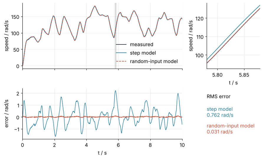
Both models have the gain, 20.01 and 20.00 rad/s per V against the true 20.00. Only the random-input model has the dynamics: a fast time constant of 0.0498 s against 0.0500 s, where the step model has 0.0399 s and a slow one of 0.2648 s instead of 0.2500 s. The step characteristics barely show it, a rise time of 0.59 s against 0.57 s and a settling time of 1.09 s against 1.04 s, because rise and settling are what a step measures. On the validation record the two predictions lie on top of each other at full scale. The zoom on the right, around 5.83 s where the step model misses most, pulls them apart: the step model runs about 2 rad/s above the measurement, the random-input model on it. The errors below show it over the whole record: the step model's swings with every change of voltage, by up to 2.20 rad/s with an RMS of 0.762 rad/s, while the random-input model's stays at the sensor noise, never above 0.10 rad/s and with an RMS of 0.031 rad/s.
Where it shows up
The motor on the bench is one case of a routine that runs through engineering and beyond: drive a system with a chosen input, log its response, fit a low-order model, and check it on a record the fit never saw.
- Process control. Before a PID controller for a heat exchanger or a distillation column is tuned, an engineer bumps the valve and records the response of the plant. The bump test pins down the gain and the dominant time constant, which is what the tuning rules need, and a planned Recipe on this site fits it with a first-order model plus dead time.
- Buildings. Heating power in, indoor temperature out: low-order ARX and similar models are fitted to a building's logged data and then used in model predictive control of the heating. A thermostat that switches a few times a day excites the slow response of the walls far better than the fast one of the air.
- Vehicles. The steering angle in and the yaw rate out are recorded on test drives, with steps, sine sweeps, and random steering as inputs. The sweeps and the random steering are there for the reason this page gives: a single steering step says little about how the car answers quick corrections.
- Physiology. Oxygen uptake and heart rate follow the load on a cycle ergometer with time constants of their own. Exercise physiologists drive the load with pseudo-random binary sequences to estimate them, the same coin flips with a fixed clock as on the right of the first figure.
- Seismology. A seismometer's natural period and damping are measured by driving a calibration pulse through its calibration coil and recording the response. The model is second order like the motor's, with two complex decay factors instead of two real ones, because a mass on a spring rings.
In every case the input has to carry power past the corner of the fastest time constant the model must get right; what it does not carry, the fit leaves to the noise.
Further reading
numpy.linalg.lstsqfor the fit, andscipy.signal.lfilter, whose difference equation is the ARX equation, so thatlfilter(b, a, u)simulates a fitted model. The python-control documentation forcontrol.tfwith a sample timedt.- Ljung, System Identification: Theory for the User, 2nd edition, Prentice Hall, 1999, for output-error and instrumental-variable methods and the bias of ARX. Söderström and Stoica, System Identification, Prentice Hall, 1989.
- Related tutorials on this site: Least squares: what a fit minimizes, and why the residuals are squared, The Fourier transform: asking a signal how much of each frequency it contains, python-control from the ground up: a car's suspension with a worn damper, Filtering with scipy.signal: mains hum and noise out of an ECG, which designs filters and applies them with
filtfilt, Overfitting: why the model that fits its data best predicts worst, The Kalman filter: a battery's charge from a drifting current and noisy voltage, which estimates a state when the model is known. Planned: a Recipe that fits a process step test with a first-order model plus dead time, and this tutorial in Julia. - Download the notebook. It was executed with the library versions in the header.