Wavelet denoising with PyWavelets: remove the noise, keep the steps

The problem: steps in a noisy record

Here is one second of a record, 2,048 samples at 2,048 Hz, that jumps between levels eleven times under white noise: a patch-clamp current with channels opening and closing, a sensor switching state. The 4th-order Butterworth low-pass of Filtering with scipy.signal, with its cutoff tuned against the true signal, brings the RMS error from 1.00 to 0.73 in units of the noise σ. Its worst error is 6.3 σ, at a step. A step holds high frequencies too, and the low-pass removes them along with the noise. Wavelet denoising with PyWavelets brings the same record to 0.23 σ, with a worst error of 2.0 σ, and it never looks at the truth.

The idea fits in two sentences. In the discrete wavelet transform a step becomes a few large coefficients, while white noise becomes many small ones spread evenly over all of them. Set the small ones to zero, transform back, and the steps survive while most of the noise does not. The wavelet transform tutorial explains what a wavelet is with the continuous transform; this one uses the discrete transform, which PyWavelets computes with pywt.wavedec.

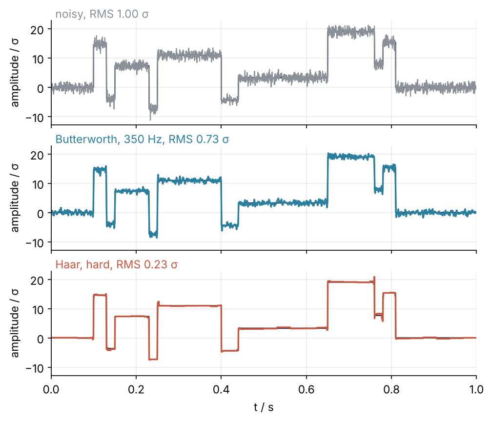
From top to bottom: the noisy record, the best low-pass, and the wavelet result, each drawn over the true signal. Step 6 draws this figure.

Setup

The test signals are Blocks and Bumps from Donoho and Johnstone's 1994 paper that introduced the method: eleven steps, and eleven narrow peaks at the same positions \(t_j\). Each is a sum of shapes,

with heights \(h_j\), a step \(K(x) = (1 + \operatorname{sgn} x)/2\) for Blocks, and a peak \(K(x) = (1 + |x|)^{-4}\) of width \(w_j\) for Bumps. Both are scaled to a standard deviation of 7 and get Gaussian noise of standard deviation 1, the paper's signal-to-noise ratio, so every amplitude below is in units of the noise σ.

import numpy as np
import matplotlib.pyplot as plt
import pywt
from scipy import signal

plt.rcParams.update({
    "figure.figsize": (7, 3.6), "figure.dpi": 110,
    "axes.spines.top": False, "axes.spines.right": False,
    "axes.grid": True, "grid.alpha": 0.25,
    "font.size": 11, "lines.linewidth": 1.8,
})
INK, ACCENT, SECOND, MUTED = "#1f2a44", "#c8553d", "#2a7f9e", "#8a8f98"

N, FS = 2048, 2048.0                       # one second of samples, in Hz
t = np.arange(N) / FS

# Donoho and Johnstone, Biometrika 81, 425 (1994)
T_J = np.array([0.10, 0.13, 0.15, 0.23, 0.25, 0.40, 0.44, 0.65, 0.76, 0.78, 0.81])
H_BLOCKS = np.array([4, -5, 3, -4, 5, -4.2, 2.1, 4.3, -3.1, 2.1, -4.2])
H_BUMPS = np.array([4, 5, 3, 4, 5, 4.2, 2.1, 4.3, 3.1, 5.1, 4.2])
W_BUMPS = np.array([0.005, 0.005, 0.006, 0.01, 0.01, 0.03, 0.01, 0.01, 0.005, 0.008, 0.005])

def blocks(t):
    x = t[:, None] - T_J
    f = (H_BLOCKS * (1 + np.sign(x)) / 2).sum(axis=1)
    return 7 * f / f.std()

def bumps(t):
    x = np.abs(t[:, None] - T_J) / W_BUMPS
    f = (H_BUMPS * (1 + x) ** -4).sum(axis=1)
    return 7 * f / f.std()

def rms(a, b):
    return np.sqrt(np.mean((a - b) ** 2))

f_blocks, f_bumps = blocks(t), bumps(t)
rng = np.random.default_rng(0)
y_blocks = f_blocks + rng.standard_normal(N)    # Blocks first: the order fixes the numbers below
y_bumps = f_bumps + rng.standard_normal(N)

print(f"N = {N}, std of the signals: Blocks {f_blocks.std():.2f}, Bumps {f_bumps.std():.2f}")
print(f"RMS error of the noisy records: Blocks {rms(y_blocks, f_blocks):.2f}, Bumps {rms(y_bumps, f_bumps):.2f}")

N = 2048, std of the signals: Blocks 7.00, Bumps 7.00
RMS error of the noisy records: Blocks 1.00, Bumps 0.99

Step 1: Decompose the signal with pywt.wavedec

One level of the discrete transform is a pair of filters of the kind the prerequisite designed. A low-pass and a high-pass filter run over the signal, and of each output only every second sample is kept. The 2,048 samples become 1,024 approximation coefficients, a coarse copy of the signal, and 1,024 detail coefficients, what the coarse copy misses. The next level does the same to the approximation. With an orthogonal wavelet (Haar, the Daubechies and the symlet wavelets all are) and mode="periodization", the whole transform is an orthogonal matrix, a rotation in 2,048 dimensions. It keeps lengths, so it keeps energy, and it turns white noise of standard deviation σ into white noise of the same σ. Steps 2 and 3 rely on that.

The filters reach past the ends of the record, and mode decides what they find there. "periodization" wraps the record around and returns exactly 2,048 coefficients. The default, "symmetric", mirrors the record at its ends and adds a few coefficients per level, so the rotation picture does not hold for it. Blocks and Bumps start and end at zero, so the steps below wrap them; the first pitfall shows what a record with ends that differ needs. Six levels, for now; Step 5 says how to choose the number.

coeffs = pywt.wavedec(y_blocks, "haar", level=6, mode="periodization")
names = ["cA6"] + [f"cD{j}" for j in range(6, 0, -1)]
print("  ".join(f"{n} {len(c)}" for n, c in zip(names, coeffs)))

energy = np.array([np.sum(c**2) for c in coeffs])
print(f"share of the energy in cA6: {energy[0] / energy.sum():.2f}")
print(f"energy of coefficients / energy of signal: {energy.sum() / np.sum(y_blocks**2):.12f}")

# sym8's 16-sample filter reaches far past the ends, so the extra coefficients show
n_sym = sum(len(c) for c in pywt.wavedec(y_bumps, "sym8", level=6))   # default mode="symmetric"
print(f"sym8 with mode='symmetric': {n_sym} coefficients for {N} samples")

cA6 32  cD6 32  cD5 64  cD4 128  cD3 256  cD2 512  cD1 1024
share of the energy in cA6: 0.89
energy of coefficients / energy of signal: 1.000000000000
sym8 with mode='symmetric': 2135 coefficients for 2048 samples

The list runs coarse first: the approximation cA6 with 32 coefficients, then the details from cD6 to the finest, cD1, with 1,024. The 32 coarse coefficients carry 89 % of the energy, and the total energy is kept to twelve digits. With sym8, a smooth wavelet of Step 5 whose filter of 16 samples reaches far past the ends, and the default mode, Bumps gets 2,135 coefficients for its 2,048 samples.

Step 2: Look at the coefficients level by level

Draw every detail coefficient as a vertical line at the time it describes, one row per level, all rows on the same scale:

Copy

ROW, CLIP = 32, 15                                  # rows 32 sigma apart; taller lines are clipped
fig, ax = plt.subplots(figsize=(7, 4.5))
for j in range(1, 7):
    d = coeffs[-j]
    tc = (np.arange(len(d)) + 0.5) * 2**j / FS      # the time each coefficient describes
    base = -(j - 1) * ROW
    ax.vlines(tc, base, base + np.clip(d, -CLIP, CLIP), color=INK, lw=1.0)
    ax.annotate(f"max {np.abs(d).max():.1f}", (1.01, base), xycoords=("axes fraction", "data"),
                va="center", color=INK)             # the true height of the tallest, clipped or not
for tj in T_J:
    ax.axvline(tj, color=MUTED, ls="--", lw=1, zorder=0)
ax.set(xlabel="t / s", ylabel=f"detail coefficient / σ, rows {ROW} apart", xlim=(0, 1),
       ylim=(-5 * ROW - CLIP - 2, CLIP + 2))
ax.set_yticks([-(j - 1) * ROW for j in range(1, 7)], [f"level {j}" for j in range(1, 7)])
ax.grid(False)
plt.show()

for j in range(6, 0, -1):
    print(f"level {j}: largest |d| = {np.abs(coeffs[-j]).max():5.1f} σ")

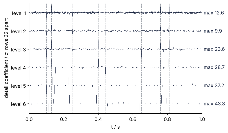
level 6: largest |d| =  43.3 σ
level 5: largest |d| =  37.2 σ
level 4: largest |d| =  28.7 σ
level 3: largest |d| =  23.6 σ
level 2: largest |d| =   9.9 σ
level 1: largest |d| =  12.6 σ

At every level the large coefficients sit at the dashed lines, the eleven steps. Between them lies a carpet of noise of the same height in every row: the rotation of Step 1 at work. The largest coefficient is 43 σ at level 6 and still 9.9 σ and 12.6 σ at levels 2 and 1, against noise of 1 σ.

Step 3: Estimate the noise from the finest level

The finest level, cD1, holds 1,024 coefficients, and almost all of them are noise. The few that sit on steps inflate the standard deviation, but they barely move the median of the absolute values. For a standard normal variable half the values of \(|Z|\) lie below 0.6745, so the noise estimate is \(\hat\sigma = \operatorname{median}(|d_1|)/0.6745\), the median absolute deviation. From it follows the universal threshold of Donoho and Johnstone,

The largest of \(N\) independent noise values stays below \(\lambda\) with a probability that tends to one as \(N\) grows. Here \(N\) is the record length, the number of noise values the rotation hands to the coefficients: 2,016 details and 32 coarse ones.

cD1 = coeffs[-1]
sigma = np.median(np.abs(cD1)) / 0.6745
lam = sigma * np.sqrt(2 * np.log(N))
print(f"std of cD1   {np.std(cD1):.3f}")
print(f"MAD estimate {sigma:.3f}")
print(f"threshold    {lam:.2f}   (sqrt(2 ln N) = {np.sqrt(2 * np.log(N)):.3f})")

std of cD1   1.223
MAD estimate 1.010
threshold    3.95   (sqrt(2 ln N) = 3.905)

The standard deviation reads 1.22, the MAD estimate 1.010, against a true σ of 1. The threshold is 3.95: anything smaller is treated as noise.

Step 4: Threshold hard and soft, and transform back

pywt.threshold(d, lam, mode="hard") keeps every coefficient whose magnitude reaches λ and sets the rest to zero. mode="soft" does the same and also shrinks every survivor toward zero by λ. The default is soft, so always spell the mode out. Only the detail levels are thresholded: cA6 carries 89 % of the energy and holds the signal's mean levels, not noise. pywt.waverec then rebuilds the signal, with the same wavelet and mode; the boundary argument and the trim to len(y) are for the first pitfall. The whole chain fits in one function:

def denoise(y, wavelet, mode, level=6, scale=1.0, boundary="periodization"):
    """Threshold the details at scale times the universal threshold and rebuild."""
    coeffs = pywt.wavedec(y, wavelet, level=level, mode=boundary)
    sigma = np.median(np.abs(coeffs[-1])) / 0.6745
    lam = scale * sigma * np.sqrt(2 * np.log(len(y)))
    details = [pywt.threshold(d, lam, mode=mode) for d in coeffs[1:]]
    return pywt.waverec([coeffs[0]] + details, wavelet, mode=boundary)[:len(y)]

n_kept = sum(np.sum(np.abs(d) >= lam) for d in coeffs[1:])
print(f"Blocks, haar: {n_kept} of {N - len(coeffs[0])} detail coefficients survive")

peaks = np.round(T_J * FS).astype(int)          # sample index of each peak center
for mode in ["hard", "soft"]:
    x_blocks = denoise(y_blocks, "haar", mode)
    x_bumps = denoise(y_bumps, "sym8", mode)
    print(f"{mode}: RMS Blocks {rms(x_blocks, f_blocks):.2f}, Bumps {rms(x_bumps, f_bumps):.2f};"
          f"  mean error at the Bumps peaks {np.mean(x_bumps[peaks] - f_bumps[peaks]):+.1f}")
print(f"soft at lambda/2: RMS Blocks {rms(denoise(y_blocks, 'haar', 'soft', scale=0.5), f_blocks):.2f}, "
      f"Bumps {rms(denoise(y_bumps, 'sym8', 'soft', scale=0.5), f_bumps):.2f}")

Blocks, haar: 48 of 2016 detail coefficients survive
hard: RMS Blocks 0.23, Bumps 0.55;  mean error at the Bumps peaks -1.7
soft: RMS Blocks 0.64, Bumps 1.03;  mean error at the Bumps peaks -7.9
soft at lambda/2: RMS Blocks 0.39, Bumps 0.63

Of 2,016 detail coefficients, 48 survive. Hard thresholding brings Blocks from 1.00 to 0.23 and Bumps, with the smooth wavelet sym8 that Step 5 explains, from 0.99 to 0.55. Soft thresholding gives 0.64 and 1.03, and on Bumps that is worse than doing nothing. The zoom on the first five steps shows why:

Copy

fig, axes = plt.subplots(2, 1, sharex=True, figsize=(7, 4.4))
zoom = (t >= 0.08) & (t <= 0.30)
for ax, mode in zip(axes, ["hard", "soft"]):
    x = denoise(y_blocks, "haar", mode)
    ax.plot(t[zoom], y_blocks[zoom], "o", color=MUTED, ms=2)
    ax.plot(t[zoom], f_blocks[zoom], color=INK, lw=1.2)
    ax.plot(t[zoom], x[zoom], color=ACCENT)
    ax.text(0.01, 1.0, f"{mode}, RMS {rms(x, f_blocks):.2f} σ", transform=ax.transAxes,
            va="bottom", color=ACCENT)
    ax.set(ylabel="amplitude / σ")
axes[-1].set(xlabel="t / s", xlim=(0.08, 0.30))
plt.show()

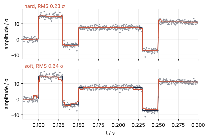
Soft thresholding pulls every step and every peak in. Each surviving coefficient on each level loses λ, and at a feature these losses add up: the Bumps peaks come out 7.9 σ low on average, against 1.7 σ with hard thresholding. At the universal threshold that bias outweighs the noise it removes. With the universal threshold use hard thresholding, which keeps heights. Soft thresholding belongs with a smaller threshold: at λ/2 it gives 0.39 and 0.63, closing most of the gap, and BayesShrink in the Variations picks one per level.

Step 5: Choose the wavelet and the decomposition level

dbN (Daubechies) and symN (symlets, a more symmetric variant of the same family) have N vanishing moments and filters of 2N samples: the detail filter gives exactly zero on any polynomial of degree below N. Haar (db1) ignores only constants, so the slope of a peak leaks into its details. sym8 ignores polynomials up to degree 7, so a smooth peak costs few coefficients, while a step costs more because the 16-sample filter straddles it longer. The two shapes, from pywt.Wavelet(name).wavefun(), span one sample less than their filters:

Copy

fig, axes = plt.subplots(1, 2, sharey=True, figsize=(7, 2.4))
for ax, name in zip(axes, ["haar", "sym8"]):
    w = pywt.Wavelet(name)
    phi, psi, x = w.wavefun(level=8)
    ax.plot(x, psi, color=INK)
    ax.text(0.01, 1.0, f"{name}, {w.vanishing_moments_psi} vanishing moment{'s' * (w.vanishing_moments_psi > 1)}",
            transform=ax.transAxes, va="bottom", color=INK)
    ax.set(xlabel="support / filter samples")
axes[0].set(ylabel="ψ")
plt.show()

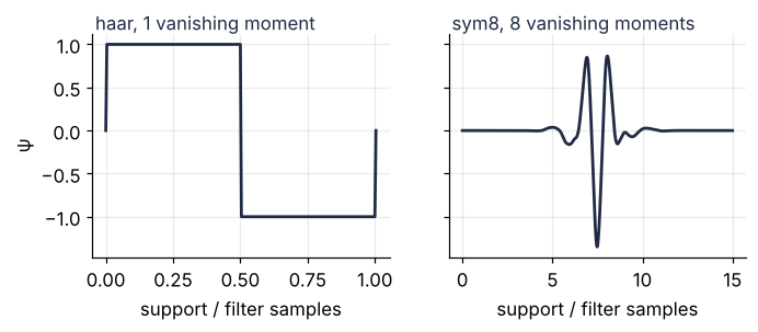
The rule is a wavelet that looks like the features: Haar for steps, a smooth one of moderate length for peaks. Checked against the truth:

print("wavelet  moments  filter  sigma(Bumps)  RMS Blocks  RMS Bumps")
for name in ["haar", "db2", "sym4", "sym8"]:
    w = pywt.Wavelet(name)
    s = np.median(np.abs(pywt.wavedec(y_bumps, name, level=6, mode="periodization")[-1])) / 0.6745
    print(f"{name:7s}  {w.vanishing_moments_psi:7d}  {w.dec_len:6d}  {s:12.2f}"
          f"  {rms(denoise(y_blocks, name, 'hard'), f_blocks):10.2f}  {rms(denoise(y_bumps, name, 'hard'), f_bumps):9.2f}")

wavelet  moments  filter  sigma(Bumps)  RMS Blocks  RMS Bumps
haar           1       2          1.09        0.23       0.76
db2            2       4          1.05        0.42       0.50
sym4           4       8          1.00        0.46       0.51
sym8           8      16          0.99        0.56       0.55

The wrong wavelet is expensive: 0.56 instead of 0.23 on Blocks with sym8, 0.76 instead of 0.55 on Bumps with Haar. Haar even misjudges the noise on Bumps, 1.09 where sym8 reads 0.99, because the peaks' slopes leak into cD1. The three smooth wavelets land within 0.05 of each other on Bumps, so "moderate" means 4 to 16 filter samples; sym8 is Donoho and Johnstone's choice. On the tallest peaks:

Copy

fig, axes = plt.subplots(2, 1, sharex=True, figsize=(7, 4.4))
zoom = (t >= 0.745) & (t <= 0.825)
for ax, name in zip(axes, ["haar", "sym8"]):
    x = denoise(y_bumps, name, "hard")
    ax.plot(t[zoom], y_bumps[zoom], "o", color=MUTED, ms=2)
    ax.plot(t[zoom], f_bumps[zoom], color=INK, lw=1.2)
    ax.plot(t[zoom], x[zoom], color=ACCENT)
    ax.text(0.01, 1.0, f"{name}, RMS {rms(x, f_bumps):.2f} σ", transform=ax.transAxes,
            va="bottom", color=ACCENT)
    ax.set(ylabel="amplitude / σ")
axes[-1].set(xlabel="t / s", xlim=(0.745, 0.825))
plt.show()

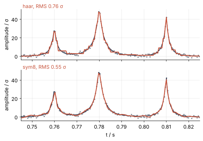
The level matters because the coarse coefficients are never thresholded, so any noise left in them passes straight into the result. Each level more moves half of what remains into thresholded details:

for label, y, f, name in [("Blocks, haar", y_blocks, f_blocks, "haar"), ("Bumps, sym8 ", y_bumps, f_bumps, "sym8")]:
    print(label, " ".join(f"{rms(denoise(y, name, 'hard', level=L), f):.2f}" for L in range(1, 8)))
print("deepest level for sym8:", pywt.dwt_max_level(N, pywt.Wavelet("sym8").dec_len))

Blocks, haar 0.70 0.51 0.37 0.30 0.25 0.23 0.23
Bumps, sym8  0.72 0.61 0.55 0.53 0.54 0.55 0.55
deepest level for sym8: 7

Blocks falls from 0.70 at level 1 to 0.23 at level 6; Bumps reaches 0.55 at level 3 and stays within 0.02 of it. Decompose until about 32 coarse coefficients remain, a level of about \(\log_2 N - 5\), and never deeper than pywt.dwt_max_level(len(y), wavelet.dec_len), here 7: one level more and the coarse coefficients are fewer than the filter's samples. The table and the sweep use the truth and are only checks; the choices need only the features' shape and the record's length.

Step 6: Compare with a Butterworth low-pass

The low-pass is the one from the prerequisite, signal.butter(4, fc, fs=FS, output="sos") run forward and backward with signal.sosfiltfilt. Its cutoff is swept from 20 to 600 Hz in steps of 5 Hz and the best one kept against the truth, the most favorable case for the filter:

Copy

cutoffs = np.arange(20, 601, 5)

def best_lowpass(y, f):
    errors = [rms(signal.sosfiltfilt(signal.butter(4, fc, fs=FS, output="sos"), y), f) for fc in cutoffs]
    k = int(np.argmin(errors))
    return cutoffs[k], signal.sosfiltfilt(signal.butter(4, cutoffs[k], fs=FS, output="sos"), y)

fc_blocks, lp_blocks = best_lowpass(y_blocks, f_blocks)
fc_bumps, lp_bumps = best_lowpass(y_bumps, f_bumps)
wv_blocks, wv_bumps = denoise(y_blocks, "haar", "hard"), denoise(y_bumps, "sym8", "hard")
print(f"Blocks: low-pass {rms(lp_blocks, f_blocks):.2f} at {fc_blocks} Hz, wavelet {rms(wv_blocks, f_blocks):.2f}")
print(f"Bumps:  low-pass {rms(lp_bumps, f_bumps):.2f} at {fc_bumps} Hz, wavelet {rms(wv_bumps, f_bumps):.2f}")
print(f"largest error on Blocks: low-pass {np.abs(lp_blocks - f_blocks).max():.1f}, "
      f"wavelet {np.abs(wv_blocks - f_blocks).max():.1f}")

fig, axes = plt.subplots(3, 1, sharex=True, sharey=True, figsize=(7.5, 6.3))
panels = [(y_blocks, MUTED, f"noisy, RMS {rms(y_blocks, f_blocks):.2f} σ"),
          (lp_blocks, SECOND, f"Butterworth, {fc_blocks} Hz, RMS {rms(lp_blocks, f_blocks):.2f} σ"),
          (wv_blocks, ACCENT, f"Haar, hard, RMS {rms(wv_blocks, f_blocks):.2f} σ")]
for ax, (x, color, label) in zip(axes, panels):
    ax.plot(t, f_blocks, color=INK, lw=1.2)
    ax.plot(t, x, color=color, lw=1.0 if color == MUTED else 1.6)
    ax.text(0.01, 1.0, label, transform=ax.transAxes, va="bottom", color=color)
    ax.set(ylabel="amplitude / σ")
axes[-1].set(xlabel="t / s", xlim=(0, 1))
plt.show()

Blocks: low-pass 0.73 at 350 Hz, wavelet 0.23
Bumps:  low-pass 0.71 at 415 Hz, wavelet 0.55
largest error on Blocks: low-pass 6.3, wavelet 2.0

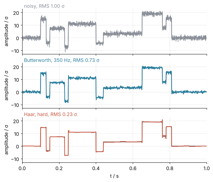
The best cutoffs are 350 Hz for Blocks and 415 Hz for Bumps, with RMS errors of 0.73 and 0.71 against 0.23 and 0.55 for the wavelets. The low-pass error sits at the steps, 6.3 σ at worst. The wavelet error is a few blips of up to 2.0 σ where a step falls inside a pair of samples that a coarse level averages together.

Pitfalls

Ends that do not match. periodization treats the record as one period of a periodic signal, so the last sample is followed by the first. A real record rarely ends where it began. Give Bumps a slow drift of 6 σ over the second and the seam becomes a step, which sym8 straddles and spreads over both ends:

drift = 6 * t                                   # the ends now differ by 6 σ
for boundary in ["periodization", "symmetric"]:
    x = denoise(y_bumps + drift, "sym8", "hard", boundary=boundary)
    e = np.abs(x - (f_bumps + drift))
    print(f"{boundary:13s}  largest error in the first and last 32 samples: {e[:32].max():.1f} σ, {e[-32:].max():.1f} σ;"
          f"  RMS {rms(x, f_bumps + drift):.2f}")
c = pywt.wavedec(y_blocks[:2001], "haar", level=6, mode="symmetric")
print("2,001 samples with mode='symmetric' come back from waverec as", len(pywt.waverec(c, "haar", mode="symmetric")))

periodization  largest error in the first and last 32 samples: 2.1 σ, 3.8 σ;  RMS 0.59
symmetric      largest error in the first and last 32 samples: 0.1 σ, 0.1 σ;  RMS 0.60
2,001 samples with mode='symmetric' come back from waverec as 2002

Wrapped, the ends are off by 2.1 σ and 3.8 σ. Mirrored, with the default mode="symmetric", there is no seam and the ends are off by 0.1 σ. The price is small: the extra coefficients make the rotation of Step 1 inexact, and the RMS error is 0.60 against 0.59. Use symmetric for a real record and trim the result to len(y), because a level of odd length rounds up and 2,001 samples come back as 2,002. Keep periodization for records whose ends match, or for Haar at a length that is a power of two, whose pairs never straddle the seam.

Thresholding the approximation too. Soft thresholding of the whole list, cA6 included, pulls the entire signal toward zero, because the coarse coefficients are the mean levels of Step 4, not noise:

c = pywt.wavedec(y_blocks, "haar", level=6, mode="periodization")
x = pywt.waverec([pywt.threshold(a, lam, mode="soft") for a in c], "haar", mode="periodization")
print(f"Blocks, soft, cA6 thresholded too: RMS {rms(x, f_blocks):.2f}  (details only: 0.64)")

Blocks, soft, cA6 thresholded too: RMS 0.76  (details only: 0.64)

The error rises from 0.64 to 0.76. Leave coeffs[0] untouched.

The result depends on where the record starts. Shift Blocks by a few samples, denoise, shift back, and the error changes:

shifted = [rms(np.roll(denoise(np.roll(y_blocks, s), "haar", "hard"), -s), f_blocks) for s in range(8)]
print("shift 0 to 7 samples:", " ".join(f"{e:.2f}" for e in shifted))

shift 0 to 7 samples: 0.23 0.22 0.21 0.24 0.23 0.20 0.26 0.26

Between 0.20 and 0.26, from the same data. Keeping every second sample makes the transform depend on where the pairs of samples begin: a step that falls inside a pair spreads over more coefficients than one between pairs. The stationary transform of the first variation skips the subsampling and removes the dependence.

Variations

• Shift-invariant denoising. The stationary transform keeps all 2,048 coefficients on every level and spreads the filters out instead of dropping samples, so it holds the decimated transform at every shift at once. Replace wavedec and waverec by pywt.swt(y, wavelet, level, trim_approx=True), which returns the same list as wavedec, and pywt.iswt; the length must be a multiple of \(2^L\). With the default norm=False the noise keeps the same σ on every level, so the same λ applies, and the error drops to 0.16 on Blocks and 0.38 on Bumps.
• One threshold per level. Estimate σ on each level with the same median, instead of on cD1 alone. That handles colored noise, whose strength differs between levels (Johnstone and Silverman, 1997).
• A data-adaptive threshold. skimage.restoration.denoise_wavelet(y, method="BayesShrink", mode="soft") chooses λ per level from the data and pairs it with soft thresholding.
• Images. pywt.wavedec2 and pywt.waverec2 do the same in two dimensions; Denoise a low-light micrograph with scikit-image applies it to a micrograph.

Cheat sheet

w = pywt.Wavelet("sym8")                                                 # haar for steps
L = min(int(np.log2(len(y))) - 5, pywt.dwt_max_level(len(y), w.dec_len))  # about 32 coarse coefficients
coeffs = pywt.wavedec(y, w, level=L, mode="symmetric")   # [cA_L, cD_L, ..., cD1]; "periodization" if the ends match
sigma = np.median(np.abs(coeffs[-1])) / 0.6745                           # noise from the finest level
lam = sigma * np.sqrt(2 * np.log(len(y)))                                # universal threshold
coeffs[1:] = [pywt.threshold(d, lam, mode="hard") for d in coeffs[1:]]   # never coeffs[0]; default is soft
x = pywt.waverec(coeffs, w, mode="symmetric")[:len(y)]                   # same wavelet and mode; trim

Further reading

• PyWavelets reference: pywt.wavedec and pywt.waverec, pywt.threshold, and pywt.swt.
• D. L. Donoho and I. M. Johnstone, Ideal spatial adaptation by wavelet shrinkage, Biometrika 81, 425 (1994), the test signals and the universal threshold.
• G. R. Lee, R. Gommers, F. Wasilewski, K. Wohlfahrt, and A. O'Leary, PyWavelets: A Python package for wavelet analysis, J. Open Source Softw. 4, 1237 (2019).
• S. Mallat, A Wavelet Tour of Signal Processing (3rd ed., Academic Press, 2009).
• D. B. Percival and A. T. Walden, Wavelet Methods for Time Series Analysis (Cambridge, 2000).
• Related tutorials on this site: Filtering with scipy.signal: mains hum and noise out of an ECG, The wavelet transform: which frequencies a signal contains, and when, Continuous wavelet transform with PyWavelets: when El Niño went quiet, Denoise a low-light micrograph with scikit-image: what each filter keeps, and The Fourier transform: asking a signal how much of each frequency it contains.
• Download the notebook. It was executed with the library versions in the header.