Ray transfer matrices in NumPy: a beam expander and a laser cavity
Afterwards you can chain ray transfer matrices in NumPy, find focal and image planes, propagate a Gaussian beam, and test a laser cavity for stability.
- Topic
- Linear algebra
- Field
- Engineering, Physics
- Libraries
matplotlib 3.11.2numpy 2.4.3
py-ray-transfer-matrices.ipynb, executed with the versions above. The download needs a free account
Run it yourself. In a terminal, this installs exactly the versions above:
pip install numpy==2.4.3 matplotlib==3.11.2 jupyterlabThe problem: widen a laser beam four times, and keep a cavity stable
A helium-neon laser gives you a beam 1 mm wide (the diameter at which the intensity has dropped to 1/e², about 13.5 %, of its value on the axis), and the microscope behind it wants 4 mm. Two lenses do it. One pair is f₁ = 50 mm and f₂ = 200 mm, 250 mm apart; the other swaps the first lens for a diverging one, f₁ = -50 mm, and fits in a tube 100 mm shorter. Which pair, and how precisely must the lenses sit? Ray transfer matrices, also called ABCD matrices, answer both with 2 x 2 matrix products.
A ray is two numbers, its height y above the optical axis and its angle θ. For small angles every element in its path, a lens or a stretch of empty space, turns (y, θ) linearly into a new (y, θ). So each element is a 2 x 2 matrix, and a whole system is the product of its elements. The same four numbers also carry a laser beam through the system, and they settle a second question: two concave mirrors face each other as a laser cavity, and for which spacings does a ray stay near the axis however often it bounces?
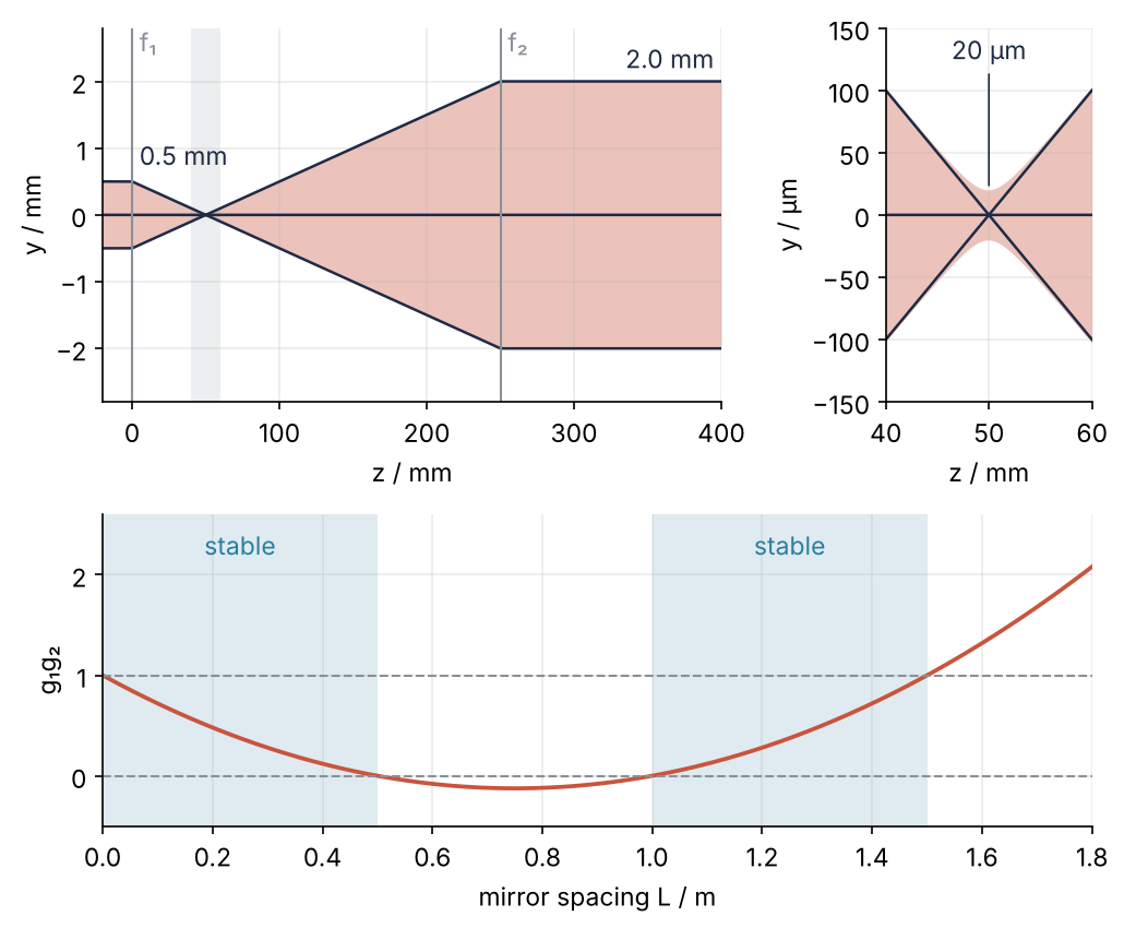
At the top is the first design, the beam as a shaded band, four times wider at the end, with one ray along the axis and two that follow its edges everywhere except near the focus, enlarged on the right, where they cross. At the bottom is the cavity, a stability measure from Step 5 against the mirror spacing, stable in the shaded ranges. Step 6 draws the figure.
Setup
All lengths are in millimeters, the wavelength included. Nothing is measured: every number below follows from the focal lengths, the mirror radii, and the wavelength.
import numpy as np
import matplotlib.pyplot as plt

lam = 633e-6     # mm, helium-neon laser; all lengths in mm
w0 = 0.5         # mm, beam radius at the first lens (1 mm diameter at 1/e²)

plt.rcParams.update({
    "figure.figsize": (7, 3.6), "figure.dpi": 110,
    "axes.spines.top": False, "axes.spines.right": False,
    "axes.grid": True, "grid.alpha": 0.25,
    "font.size": 11, "lines.linewidth": 1.8,
})
INK, ACCENT, SECOND, MUTED = "#1f2a44", "#c8553d", "#2a7f9e", "#8a8f98"

print(f"lam = {lam} mm, w0 = {w0} mm")
lam = 0.000633 mm, w0 = 0.5 mm
Step 1: Write free space, a thin lens, and a mirror as matrices
Over a distance d a ray keeps its angle, and its height grows by d θ. A thin lens of focal length f keeps the height and bends the angle by -y/f, toward the axis for f > 0; a diverging lens has f < 0. As matrices acting on the column (y, θ):
A curved mirror of radius R sends the light back. Unfold the path, drawing the reflected light as if it went on forward, and the mirror acts as a lens of focal length R/2. R > 0 is a concave mirror, which focuses; that is the convention for the whole tutorial.
def space(d):
    return np.array([[1.0, d], [0.0, 1.0]])

def lens(f):
    return np.array([[1.0, 0.0], [-1.0 / f, 1.0]])

def mirror(R):
    return lens(R / 2)                  # unfolded path, R > 0 concave

ray = np.array([0.5, 0.0])              # 0.5 mm above the axis, parallel to it
y, theta = space(50) @ lens(50) @ ray   # the lens acts first, so it stands next to the ray
print(f"y = {abs(y):.3f} mm, theta = {theta:.4f} rad")    # abs: y is -1e-17, round-off
y = 0.000 mm, theta = -0.0100 rad
A ray parallel to the axis, through a 50 mm lens and then 50 mm of space, arrives on the axis. That is what a focal length is, and the matrices know it. It gets there at -0.01 rad, the minus sign because it heads down toward the axis, and that 0.01 rad comes back in Step 4.
Step 2: Build the beam expander and read off its magnification
The light meets lens 1 first, so lens 1 acts first and stands on the right: the system matrix is lens(f2) @ space(d) @ lens(f1), the drawing read from right to left. The @ product is the one from Eigenvalues with numpy.linalg: normal modes of coupled oscillators.
kepler = lens(200) @ space(250) @ lens(50)      # two converging lenses
galileo = lens(200) @ space(150) @ lens(-50)    # diverging lens first
print("Keplerian\n", kepler)
print("Galilean\n", galileo)
Keplerian
 [[ -4.   250.  ]
 [  0.    -0.25]]
Galilean
 [[  4.   150.  ]
 [  0.     0.25]]
Each entry means something, read row by row as [[A, B], [C, D]]. A is output height per input height: -4 and +4, so both designs widen the beam four times, and the Keplerian turns it upside down. C is output angle per input height, and C = 0 says that parallel light leaves parallel; such a system is called afocal. D = 1/A, so angles shrink four times, and the wide beam spreads four times less than the narrow one did.
To draw rays you need the matrix up to every position z. upto multiplies only the elements the light has passed: space(z) @ lens(f1) between the lenses, the whole expander and then space(z - d) behind lens 2. Before lens 1, z is negative, and space(z) runs the ray backward.
def upto(z, f1, d, f2):
    if z < 0:
        return space(z)
    if z < d:
        return space(z) @ lens(f1)
    return space(z - d) @ lens(f2) @ space(d) @ lens(f1)

z = np.linspace(-20, 280, 601)
fig, axes = plt.subplots(2, 1, figsize=(7, 4.2), sharex=True)
for ax, (name, f1, d) in zip(axes, [("Keplerian", 50, 250), ("Galilean", -50, 150)]):
    for y0 in np.linspace(-0.5, 0.5, 5):
        path = [(upto(zz, f1, d, 200) @ [y0, 0.0])[0] for zz in z]
        ax.plot(z, path, color=INK, lw=1.2)
    for zl, label in [(0, "f₁"), (d, "f₂")]:
        ax.axvline(zl, color=MUTED, lw=1)
        ax.text(zl + 4, 2.3, label, color=MUTED)
    ax.text(60, 2.3, name, color=INK)
    ax.set(ylabel="y / mm", ylim=(-2.8, 2.8))
axes[1].set(xlabel="z / mm", xlim=(-20, 280))
plt.show()
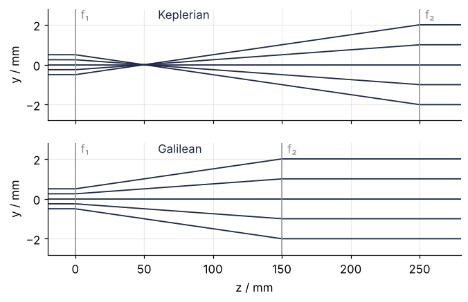
The Keplerian rays cross at 50 mm, the focal plane of lens 1, and leave inverted. The Galilean rays spread from the start, never cross, and arrive at their full width 100 mm sooner.
Step 3: Find the focal plane and the image plane from A, B, C, D
A parallel ray of height y leaves the system as (A y, C y), so it reaches the axis a distance s = -A/C behind lens 2: the back focal distance. For the expander C = 0, and the focus lies at infinity until lens 2 moves:
for delta in [1, 2, 5]:
    A, B, C, D = (lens(200) @ space(250 + delta) @ lens(50)).ravel()
    print(f"lens 2 moved {delta} mm: back focal distance {-A / C / 1000:5.1f} m")
lens 2 moved 1 mm: back focal distance  40.2 m
lens 2 moved 2 mm: back focal distance  20.2 m
lens 2 moved 5 mm: back focal distance   8.2 m
One millimeter too long and the output beam focuses 40.2 m away instead of staying parallel; 5 mm too long, and it focuses at 8.2 m. Set the spacing to a fraction of a millimeter, or put lens 2 on a slide and adjust it on the beam.
Images come from B. The output height is y' = A y + B θ, and where B = 0 it no longer depends on the input angle: every ray leaving one point arrives at one point. That is an image, with A the magnification. Adding space(s) behind the system turns B into B + s D, which is zero at s = -B/D. For a single lens between object distance \(s_o\) and image distance \(s_i\), B = 0 is the lens equation \(1/f = 1/s_o + 1/s_i\).
A, B, C, D = kepler.ravel()
s = -B / D
M = space(s) @ kepler
print(f"image of the lens-1 plane: {s:.1f} mm behind lens 2, B = {M[0, 1]:.1e}, magnification {M[0, 0]:.2f}")
image of the lens-1 plane: 1000.0 mm behind lens 2, B = 0.0e+00, magnification -4.00
The plane of lens 1 is imaged 1000 mm behind lens 2, four times enlarged and inverted. Step 4 finds the laser beam there.
Step 4: Propagate a Gaussian beam with the q parameter
A laser beam is not a bundle of rays. Its intensity falls off from the axis as a bell curve, to 1/e² at the radius w. It is narrowest at its waist, radius w₀, and widens with the distance z from it as \(w = w_0\sqrt{1 + (z/z_R)^2}\); the Rayleigh range \(z_R = \pi w_0^2/\lambda\) is the distance over which it stays roughly parallel.
z_R = np.pi * w0**2 / lam
print(f"z_R = {z_R:.0f} mm")
z_R = 1241 mm
Both lengths fit into one complex number, \(q = z + i z_R\): the distance past the waist (negative before it) plus i times the Rayleigh range. Free space adds d to q. Taken from Kogelnik and Li (Further reading), not derived: a system acts on q with the same four numbers as on rays:
Any q with positive imaginary part describes some Gaussian beam this way, and its radius follows from the two definitions, \(w^2 = (\lambda/\pi)\,|q|^2/\operatorname{Im} q\), and with Re q set to zero, its waist radius.
def propagate(M, q):
    (A, B), (C, D) = M
    return (A * q + B) / (C * q + D)

def radius(q):
    return np.sqrt(lam / np.pi * abs(q) ** 2 / q.imag)

q0 = 1j * z_R                                   # waist at lens 1
z_in = np.arange(0, 250, 0.01)
w_in = np.array([radius(propagate(upto(zz, 50, 250, 200), q0)) for zz in z_in])
i = np.argmin(w_in)
print(f"narrowest inside the Keplerian: {w_in[i] * 1000:.1f} µm at {z_in[i]:.1f} mm")

for name, M in [("Keplerian", kepler), ("Galilean", galileo)]:
    q = propagate(M, q0)
    print(f"{name:9s}  q = {q.real:6.0f} {q.imag:+.0f}i mm   waist radius {radius(1j * q.imag):.3f} mm"
          f"   z_R ratio {q.imag / z_R:.1f}")
narrowest inside the Keplerian: 20.1 µm at 49.9 mm
Keplerian  q =  -1000 +19852i mm   waist radius 2.000 mm   z_R ratio 16.0
Galilean   q =    600 +19852i mm   waist radius 2.000 mm   z_R ratio 16.0
Inside the Keplerian the beam narrows to 20.1 µm at 49.9 mm, not to a point: a waist of radius w spreads at the angle λ/(πw), so rays converging at 0.01 rad allow none narrower than λ/(π · 0.01), 20 µm.
Behind lens 2, q = -1000 + 19852i mm: the new waist lies 1000 mm on, in the image plane of Step 3, with z_R 16 times longer and the radius 2.000 mm. With C = 0 and D = 1/A the law becomes q' = A²q + AB, which puts the waist on the geometric image and scales z_R by A². A single focusing lens has C ≠ 0, and a beam with z_R far longer than f has its waist near the focal plane instead.
The Galilean delivers the same beam from a virtual waist 600 mm before lens 2, in a shorter tube. Take the Keplerian only when you want a pinhole in its 20 µm focus to clean the beam.
Step 5: Test a two-mirror cavity for stability
Unfolded, a cavity is an endless row of lenses, here mirrors of R₁ = 1000 mm and R₂ = 500 mm, L apart. One round trip from mirror 1 is mirror(R1) @ space(L) @ mirror(R2) @ space(L), and after n round trips a ray is Mⁿ times the starting ray. Write the starting ray as a sum of the two eigenvectors of M, as in the prerequisite; Mⁿ multiplies each part by μⁿ, μ its eigenvalue, so the ray stays near the axis only if both |μ| ≤ 1.
def round_trip(L, R1=1000, R2=500):
    return mirror(R1) @ space(L) @ mirror(R2) @ space(L)

print(f"det M = {np.linalg.det(round_trip(300)):.6f}")
for L in [300, 700]:
    mu = np.linalg.eigvals(round_trip(L))
    print(f"L = {L} mm: eigenvalues {np.round(mu, 3)}, |mu| = {np.round(np.abs(mu), 3)}")
det M = 1.000000
L = 300 mm: eigenvalues [-0.44+0.898j -0.44-0.898j], |mu| = [1. 1.]
L = 700 mm: eigenvalues [-1.973 -0.507], |mu| = [1.973 0.507]
Every element has determinant 1, so the product has too, and μ₁μ₂ = 1. Either both eigenvalues lie on the unit circle as a complex pair \(e^{\pm i\varphi}\) and the ray oscillates, or both are real, one exceeds 1 in magnitude, and the ray runs away. The characteristic polynomial decides: with determinant 1 it is μ² - (A + D)μ + 1 = 0, whose roots are complex exactly when |A + D| < 2, that is when 0 < (A + D + 2)/4 < 1. At 300 mm the pair is -0.44 ± 0.898i, of magnitude 1; at 700 mm the eigenvalues are -1.973 and -0.507, and a ray grows almost twofold per round trip.
Laser books write it with g = 1 - L/R for each mirror as 0 ≤ g₁g₂ ≤ 1, and the first loop checks that (A + D + 2)/4 is g₁g₂. The second walks the indices where stable is True, from np.flatnonzero, and groups them into ranges: an index right after the last one extends the range, any other starts a new one.
for L in [300, 700, 1200]:
    A, B, C, D = round_trip(L).ravel()
    g1, g2 = 1 - L / 1000, 1 - L / 500
    print(f"L = {L:4d} mm   (A + D + 2)/4 = {(A + D + 2) / 4:6.3f}   g1 g2 = {g1 * g2:6.3f}")

L_sweep = np.linspace(0, 1800, 1801)
g1g2 = (1 - L_sweep / 1000) * (1 - L_sweep / 500)
stable = (g1g2 >= 0) & (g1g2 <= 1)
ranges = []                                   # [first, last] index of each range
for i in np.flatnonzero(stable):
    if ranges and ranges[-1][1] == i - 1:
        ranges[-1][1] = i
    else:
        ranges.append([i, i])
for first, last in ranges:
    print(f"stable for L from {L_sweep[first] / 1000:.2f} to {L_sweep[last] / 1000:.2f} m")
L =  300 mm   (A + D + 2)/4 =  0.280   g1 g2 =  0.280
L =  700 mm   (A + D + 2)/4 = -0.120   g1 g2 = -0.120
L = 1200 mm   (A + D + 2)/4 =  0.280   g1 g2 =  0.280
stable for L from 0.00 to 0.50 m
stable for L from 1.00 to 1.50 m
The columns agree: the textbook condition is the trace condition. Its edges are marginal, the eigenvalues meeting at -1 or +1. This cavity holds a ray up to 0.5 m and again from 1.0 to 1.5 m.
Step 6: Draw the expander and the stability map
The beam band uses upto and radius along the Keplerian, the rays come from Step 2, and the stability map is the sweep of Step 5.
z = np.linspace(-20, 400, 4201)
w = np.array([radius(propagate(upto(zz, 50, 250, 200), q0)) for zz in z])

z_zoom = np.linspace(40, 60, 2001)                         # the focus, for the zoom panel
w_zoom = np.array([radius(propagate(upto(zz, 50, 250, 200), q0)) for zz in z_zoom])

fig = plt.figure(figsize=(7, 5.8))
grid = fig.add_gridspec(2, 2, width_ratios=[3, 1], height_ratios=[1.2, 1])
ax1, ax_zoom, ax2 = fig.add_subplot(grid[0, 0]), fig.add_subplot(grid[0, 1]), fig.add_subplot(grid[1, :])
for ax, zs, ws, scale in [(ax1, z, w, 1), (ax_zoom, z_zoom, w_zoom, 1000)]:   # scale: mm to µm in the zoom
    ax.fill_between(zs, -ws * scale, ws * scale, color=ACCENT, alpha=0.35, lw=0)   # the beam
    for y0 in [-0.5, 0.0, 0.5]:                                                      # the rays
        ax.plot(zs, [(upto(zz, 50, 250, 200) @ [y0, 0.0])[0] * scale for zz in zs], color=INK, lw=1.2)
for zl, label in [(0, "f₁"), (250, "f₂")]:
    ax1.axvline(zl, color=MUTED, lw=1)
    ax1.text(zl + 5, 2.45, label, color=MUTED)
ax1.axvspan(40, 60, color=MUTED, alpha=0.15, lw=0)          # where the zoom looks
ax1.text(5, 0.75, "0.5 mm", color=INK)
ax1.text(395, 2.2, "2.0 mm", ha="right", color=INK)
ax1.set(xlabel="z / mm", ylabel="y / mm", xlim=(-20, 400), ylim=(-2.8, 2.8))
ax_zoom.annotate("20 µm", xy=(50, 20), xytext=(50, 125), ha="center", color=INK,
                 arrowprops=dict(arrowstyle="-", color=INK, lw=0.8))
ax_zoom.set(xlabel="z / mm", ylabel="y / µm", xlim=(40, 60), ylim=(-150, 150), xticks=[40, 50, 60])

ax2.plot(L_sweep / 1000, g1g2, color=ACCENT)
for level in [0, 1]:
    ax2.axhline(level, color=MUTED, lw=1, ls="--")
for first, last in ranges:
    a, b = L_sweep[first] / 1000, L_sweep[last] / 1000
    ax2.axvspan(a, b, color=SECOND, alpha=0.15, lw=0)
    ax2.text((a + b) / 2, 2.2, "stable", ha="center", color=SECOND)
ax2.set(xlabel="mirror spacing L / m", ylabel="g₁g₂", xlim=(0, 1.8), ylim=(-0.5, 2.6))
fig.tight_layout()
plt.show()
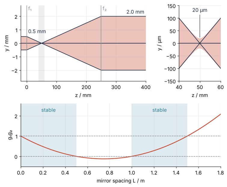
Rays and beam agree everywhere except within a few millimeters of the focus, the gray strip that the right panel enlarges: there the rays meet in a point and the beam stops at 20 µm. In the lower panel the shaded ranges are exactly where g₁g₂ lies between the two dashed lines.
Pitfalls
Multiplying in the order you read the drawing. Light goes left to right in the drawing, so it is tempting to write the matrices left to right too. That gives the expander run backward:
print("right order, A =", (lens(200) @ space(250) @ lens(50))[0, 0])
print("drawing order, A =", (lens(50) @ space(250) @ lens(200))[0, 0])
right order, A = -4.0
drawing order, A = -0.25
The "magnification" comes out as -0.25, a beam reducer. The first element the light meets goes on the right, next to the ray.
Mixing sign conventions for mirrors and angles. Some books write the mirror as [[1, 0], [2/R, 1]] with R < 0 for a concave mirror, others order the ray as (θ, y) or carry nθ, the angle times the refractive index, as the second component. Take a matrix from one book and a radius from another and a stable cavity comes out unstable: flipping the sign of R turns g = 1 - L/R into 1 + L/R, which is 2 - g. Many books also define the beam parameter by \(1/q = 1/R - i\lambda/(\pi w^2)\); it is the same q as \(z + i z_R\), but its R is the curvature of the wavefronts, not a mirror radius. Pick one book's convention and test it on two known cases before you trust a sweep: a confocal cavity, L = R₁ = R₂, has g₁g₂ = 0, and a flat-flat cavity has g₁g₂ = 1.
Trusting the matrices beyond small angles. Every matrix here assumes sin θ ≈ θ and lenses of zero thickness. A real 50 mm lens used over its full aperture adds spherical aberration, which no 2 x 2 matrix can show, and the symptom is a measured focus well above 20 µm. Keep ray angles small (the focus here converges at 0.01 rad, safely small), check a fast design with an exact ray trace through the lens surfaces, and describe what remains as a wavefront error with Zernike polynomials in NumPy: a telescope's wavefront and Strehl ratio.
Variations
- The beam a cavity holds. Solve q = (Aq + B)/(Cq + D) for the round-trip matrix, a quadratic in q. Its root with positive imaginary part is the one Gaussian beam that repeats itself after a round trip, and
radiusgives its size on each mirror. - Couple into a fiber. Replace lens 2 by a focusing lens and search over its focal length for the waist that matches the radius of the light the fiber guides, one
propagateper candidate. - Refraction and thick lenses. A flat interface from index n₁ to n₂ is [[1, 0], [0, n₁/n₂]], and a curved one adds a power term in the lower left. A thick lens is two interfaces and a space between them, the same product.
- Symbolic ABCD. The same products in SymPy give the two-lens formula and the stability condition in closed form; see SymPy from the ground up: where the pendulum's 1.74 % comes from.
Cheat sheet
space = lambda d: np.array([[1, d], [0, 1]])          # free space of length d
lens = lambda f: np.array([[1, 0], [-1 / f, 1]])      # thin lens, f < 0 diverging
mirror = lambda R: lens(R / 2)                        # unfolded, R > 0 concave
M = lens(f2) @ space(d) @ lens(f1)                    # first element met on the right
A, B, C, D = M.ravel()                                # A magnification, C = 0 afocal
s_focus, s_image = -A / C, -B / D                     # behind the last element
q = z + 1j * z_R                                      # distance past waist + i Rayleigh range
q_out = (A * q + B) / (C * q + D)                     # w² = lam/pi |q|² / Im q
stable = abs(A + D) < 2                               # round-trip matrix of a cavity
Further reading
- Saleh and Teich, Fundamentals of Photonics, the chapters on ray optics and beam optics, for the matrices and the Gaussian beam.
- Siegman, Lasers, the chapters on ray matrices and resonator stability, with a careful account of sign conventions.
- Kogelnik and Li, "Laser Beams and Resonators", Applied Optics 5, 1550 (1966), the standard review of the q parameter's ABCD law (Kogelnik, 1965) and of the g parameters (Boyd and Kogelnik, 1962).
numpy.linalg.eigvals, the NumPy reference.- Related tutorials on this site: Eigenvalues with numpy.linalg: normal modes of coupled oscillators, the prerequisite; The angular spectrum method with numpy.fft: a laser beam and a slit, a 633 nm Gaussian beam computed by diffraction instead of a matrix; The point spread function: why two points closer than 0.61 λ/NA merge, the diffraction-limited focus behind the third pitfall; Zernike polynomials in NumPy: a telescope's wavefront and Strehl ratio. Planned: the same tutorial in Julia.
- Download the notebook. It was executed with the library versions in the header.