The point spread function: why two points closer than 0.61 λ/NA merge (Python)

The question

A single fluorescent molecule is a few nanometers across. Put it under an oil objective with a numerical aperture of 1.4, let it glow green at 520 nm, and its image on the camera is a spot about half a micrometer wide. That spot is the point spread function (PSF) of the microscope, and for a round lens it has a shape with a name, the Airy pattern. The numerical aperture is NA = n sin α, the refractive index of the immersion oil times the sine of the half-angle of the light cone the objective accepts. Here is what the camera records for one molecule and for two pairs:

Show code

import numpy as np
import matplotlib.pyplot as plt
from matplotlib.colors import LogNorm, ListedColormap
from scipy.special import j1, jn_zeros

plt.rcParams.update({
    "figure.figsize": (8, 2.8), "figure.dpi": 110,
    "axes.spines.top": False, "axes.spines.right": False,
    "axes.grid": True, "grid.alpha": 0.25,
    "font.size": 11, "lines.linewidth": 1.8,
})
INK, ACCENT, SECOND, MUTED = "#1f2a44", "#c8553d", "#2a7f9e", "#8a8f98"

wavelength, NA = 520.0, 1.4                      # nm, oil objective
RAYLEIGH = jn_zeros(1, 1)[0] / np.pi             # first dark ring, in units of λ/D


def airy(u):
    """Airy intensity with peak 1 at a distance u in units of λ/D (λ/(2 NA) in the sample)."""
    v = np.pi * np.abs(np.asarray(u, float))
    out = np.ones_like(v)
    out[v > 0] = (2 * j1(v[v > 0]) / v[v > 0])**2
    return out


# Synthetic, so the answer can be checked; pretend you have not seen this cell.
rng = np.random.default_rng(281)
pixel, peak, background = 40.0, 400, 10          # nm per pixel in the sample, photons
c = (np.arange(40) - 19.5) * pixel
X, Y = np.meshgrid(c, c)

def camera(separation):
    centers = [0.0] if separation == 0 else [-separation / 2, separation / 2]
    expected = background + sum(peak * airy(np.hypot(X - x0, Y) * 2 * NA / wavelength) for x0 in centers)
    return rng.poisson(expected)

fig, axes = plt.subplots(1, 3)
for ax, sep, label in zip(axes, [0, 400, 150], ["one molecule", "400 nm apart", "150 nm apart"]):
    ax.imshow(camera(sep), cmap="cividis", vmin=0, vmax=1.1 * (peak + background))
    ax.set_axis_off()
    ax.text(1, 2, label, color="white", va="top")
axes[0].plot([2, 2 + 500 / pixel], [36, 36], color="white", lw=3)
axes[0].text(2 + 250 / pixel, 34.5, "500 nm", color="white", ha="center")
plt.show()

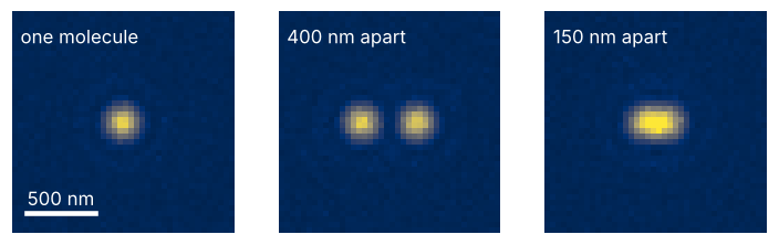
Simulated camera images of one fluorescent molecule and of pairs 400 nm and 150 nm apart. The single molecule is a spot about 500 nm wide; the 400 nm pair shows two spots, the 150 nm pair one oval spot.

Two things are obvious. The spot is about a hundred times wider than the molecule that made it, and every molecule makes the same spot. The pair 400 nm apart is two spots. The pair 150 nm apart is one spot, slightly oval, and nobody shown this image without the label would guess that it holds two molecules.

Less obvious: why is the spot this size, and why is it the same for every objective with NA 1.4 in green light, whoever made it? The textbook rule is that two molecules closer than about 0.61 λ/NA, 227 nm here, merge into one spot. Why does the same rule, written as 1.22 λ/D in angle with D the diameter of the mirror, hold the Hubble Space Telescope to 0.052″ at 500 nm? And where exactly is the line between two and one? The rest of this page is about where these numbers come from, and which part of them is physics and which is convention.

The idea: the lens adds up the waves that cross its aperture

Light from a distant point arrives at the lens as a plane wave that fills the aperture. A perfect lens delays each part of the wave just enough that all of it arrives in step at one point, the focus. The pattern around that point is the far field of the aperture, brought from infinity into the focal plane; The angular spectrum method with numpy.fft: a laser beam and a slit shows when a field counts as far.

Now look a little off the axis, in a direction θ. A wave crossing the aperture at a position x travels farther than one through the center, by x sin θ, which is x θ for small angles: a phase delay of 2π x θ/λ. The field in that direction is the sum of the unit phasors exp(−2πi x θ/λ) over the whole aperture. That is the probe of The Fourier transform: asking a signal how much of each frequency it contains, now in space instead of time. The aperture is the signal, and each direction asks how much of the spatial frequency θ/λ it contains.

For a slit of width D the answer is quick. At θ = λ/D the phase runs through one full turn across the slit, each half cancels the other, and the field is zero. A circle is different. At a position x it is not one point that counts but the whole chord of the circle there, and the chords are short near the rim. The rim gets less weight and the center more, so the cancellation needs a steeper phase ramp. Both apertures are symmetric about their center, so the sine parts of the phasors cancel in pairs and a cosine probe is enough. Here is the chord as a weight, the cosine probe, and their product, at three angles:

x = np.linspace(-0.5, 0.5, 2001)                     # position across the pupil, in units of D
chord = 2 * np.sqrt(np.clip(0.25 - x**2, 0, None))   # length of the circle's chord at x
slit = np.ones_like(x)

def probe_average(weight, theta):
    """Weighted average of the cosine probe at angle theta (in λ/D); 1 on the axis."""
    return np.trapezoid(weight * np.cos(2 * np.pi * x * theta), x) / np.trapezoid(weight, x)

fig, axes = plt.subplots(3, 1, figsize=(8, 6.5), sharex=True)
for ax, theta in zip(axes, [0.5, 1.0, RAYLEIGH]):
    probe = np.cos(2 * np.pi * x * theta)
    ax.plot(x, chord, color=INK, label="chord")
    ax.plot(x, probe, color=SECOND, lw=1, label="probe")
    ax.fill_between(x, 0, chord * probe, color=ACCENT, alpha=0.35, lw=0, label="product")
    ax.set(ylabel="weight / center value", ylim=(-1.15, 1.6))
    note = f"θ = {theta:.2f} λ/D    circle {probe_average(chord, theta):+.3f}    slit {probe_average(slit, theta):+.3f}"
    ax.text(0.99, 0.97, note.replace("-", "−"), transform=ax.transAxes, ha="right", va="top")
axes[0].legend(frameon=False, loc="lower left", ncol=3)
axes[-1].set_xlabel("x / D")
plt.show()

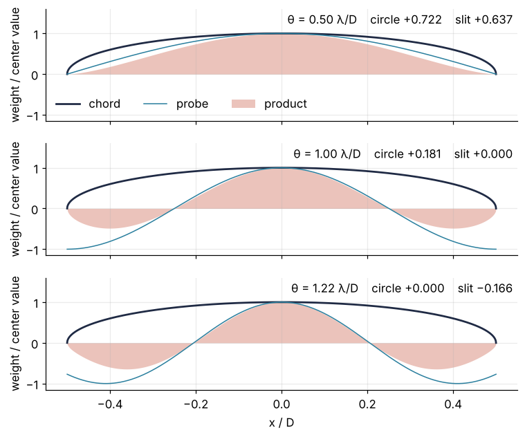
Three stacked panels at angles 0.5, 1.0, and 1.22 λ/D: the chord length across a circular pupil, a cosine probe, and their product as a filled area, against position x/D. The circle averages 0.722, 0.181, and 0.000; a slit averages 0.637, 0.000, and −0.166.

At 0.5 λ/D the product is mostly positive, and the average is 0.722 of its value on the axis. At λ/D the slit has gone dark, but the circle still averages 0.181: the short chords at the rim cannot cancel the long ones in the middle. Only at 1.22 λ/D does the circle reach zero, its first dark ring, while the slit is already past its zero at −0.166. The 1.22 in every resolution formula is the shape of a circle and nothing more.

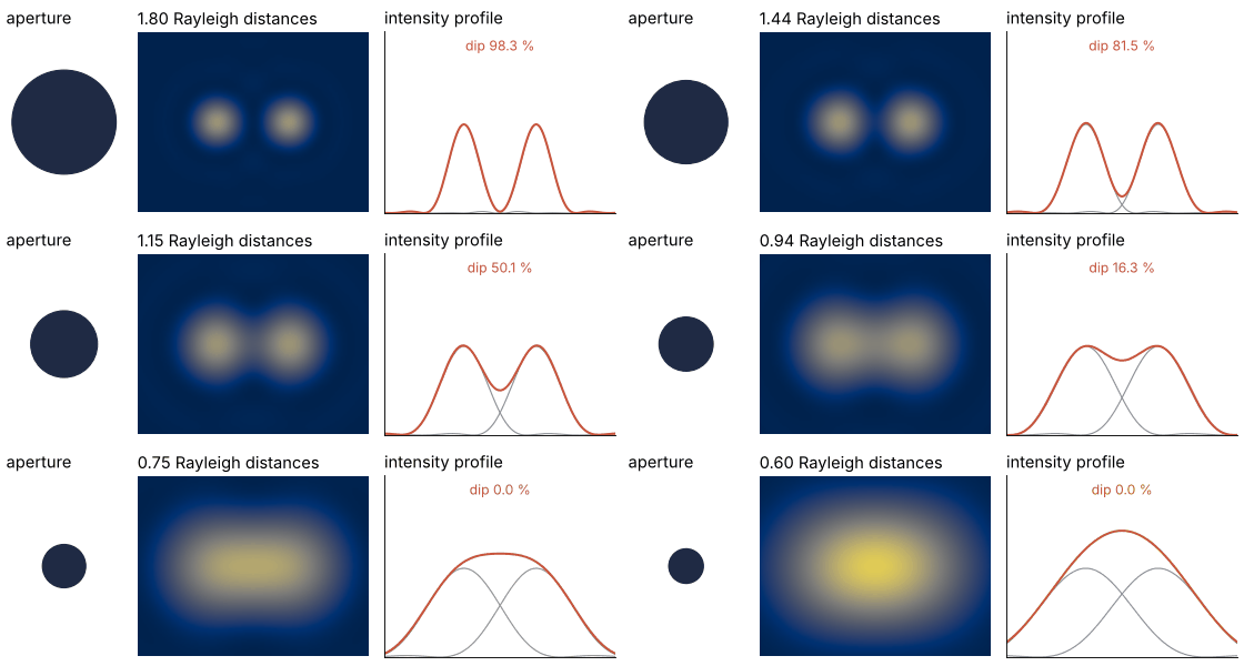
Two molecules, or two stars, emit independently, with no fixed phase between them, so on the camera their intensities add, not their fields. An image formed this way is called incoherent, and fluorescence microscopy and astronomy both work with it. Rayleigh's rule for when two such points count as resolved is that the peak of one sits on the first dark ring of the other, 1.22 λ/D away, the angle the figure just found. That separation is the Rayleigh distance. Here the aperture shrinks while the two points stay where they are:

Animation: a circular aperture shrinks while two point sources stay a fixed distance apart, from 1.8 to 0.6 Rayleigh distances. Their Airy disks grow and merge, and the dip in the intensity profile between them shrinks to zero.

Show code

"""Aperture sweep: a circular aperture shrinks while two point sources stay a fixed distance apart.

Renders ../../assets/aperture-sweep.gif. Left: the aperture. Middle: the image of the two
points, the sum of two exact Airy patterns. Right: the intensity along the line through
both points. As the aperture shrinks, the Rayleigh distance 1.22 λ/D grows, so the fixed
separation goes from 1.8 to 0.6 Rayleigh distances. Run it from any directory:

    python scene.py
"""
from pathlib import Path

import numpy as np
import matplotlib.pyplot as plt
from matplotlib.animation import FuncAnimation, PillowWriter
from matplotlib.patches import Circle
from scipy.special import j1, jn_zeros

OUT = Path(__file__).resolve().parents[2] / "assets" / "aperture-sweep.gif"
INK, ACCENT, SECOND, MUTED = "#1f2a44", "#c8553d", "#2a7f9e", "#8a8f98"
plt.rcParams.update({"font.size": 11})
RAYLEIGH = jn_zeros(1, 1)[0] / np.pi                 # first dark ring, 1.2197 in units of λ/D


def airy(u):
    """Airy intensity, peak 1, at a distance u in units of λ/D."""
    v = np.pi * np.abs(u) + 1e-12                    # the limit at v = 0 is 1
    return (2 * j1(v) / v) ** 2


# ---- lengths in units of the separation s of the two points, which never changes
x = np.linspace(-1.6, 1.6, 129)
y = np.linspace(-1.25, 1.25, 101)               # 3.2 : 2.5, the shape of the middle panel
X, Y = np.meshgrid(x, y)

# ---- the sweep: separation in Rayleigh distances, 1.8 down to 0.6 on a log scale
ratios = 1.8 * (0.6 / 1.8) ** np.linspace(0, 1, 80)
ratios = np.concatenate([ratios, np.full(12, ratios[-1])])   # hold the last frame

fig, (ax_pup, ax_img, ax_prof) = plt.subplots(1, 3, figsize=(7, 2.5), dpi=80,
                                              width_ratios=[0.8, 1.6, 1.6])
fig.subplots_adjust(left=0.01, right=0.99, top=0.86, bottom=0.04, wspace=0.08)
box = ax_pup.get_position()                          # pupil limits with the shape of its axes, so circles stay round
half_height = 0.5 * box.height * fig.get_figheight() / (box.width * fig.get_figwidth())


def update(ratio):
    rayleigh = 1 / ratio                             # the Rayleigh distance in units of s
    scale = RAYLEIGH / rayleigh                      # λ/D per unit of s
    left = airy(np.hypot(X + 0.5, Y) * scale)
    right = airy(np.hypot(X - 0.5, Y) * scale)
    a, b = airy((x + 0.5) * scale), airy((x - 0.5) * scale)
    total = a + b
    dip = 1 - total[x.size // 2] / total.max()

    for ax in (ax_pup, ax_img, ax_prof):
        ax.clear()
    ax_pup.set_axis_off()
    ax_pup.add_patch(Circle((0, 0), 0.45 * ratio / 1.8, color=INK))   # diameter ∝ D
    ax_pup.set(xlim=(-0.5, 0.5), ylim=(-half_height, half_height))
    ax_pup.set_title("aperture", loc="left")

    ax_img.set_axis_off()
    ax_img.imshow(left + right, extent=(x[0], x[-1], y[0], y[-1]), cmap="cividis",
                  vmin=0, vmax=1.6, interpolation="bilinear")
    ax_img.set_title(f"{ratio:.2f} Rayleigh distances", loc="left")

    ax_prof.plot(x, a, color=MUTED, lw=1)
    ax_prof.plot(x, b, color=MUTED, lw=1)
    ax_prof.plot(x, total, color=ACCENT, lw=1.8)
    ax_prof.text(0, 1.98, f"dip {100 * dip:.1f} %", ha="center", va="top", color=ACCENT)
    ax_prof.set(xlim=(x[0], x[-1]), ylim=(0, 2.05), xticks=[], yticks=[])
    ax_prof.spines[["top", "right"]].set_visible(False)
    ax_prof.set_title("intensity profile", loc="left")


anim = FuncAnimation(fig, update, frames=ratios)
anim.save(OUT, writer=PillowWriter(fps=12))
print(f"{OUT.name}: {OUT.stat().st_size / 1e6:.2f} MB")

As the aperture shrinks, each Airy disk grows and the dip between the peaks gets shallower. At one Rayleigh distance the dip is still plainly there, about a quarter of the peak height. It vanishes only at 0.78 of that distance, and the Formalization derives both numbers.

A hole in the pupil and a bent wavefront

The aperture as the light sees it, with what blocks it and the phase it adds, is the pupil, and real pupils are rarely clear disks. A reflecting telescope's secondary mirror blocks the center of the primary, 0.33 of the diameter in Hubble. A lens with imperfect surfaces adds a phase: the wavefront arriving at the focus departs from the perfect sphere by a distance W that changes across the pupil, the wavefront error. Its root mean square over the pupil, in wavelengths, is the one number quoted for it, and at λ/4 RMS the light from a typical part of the pupil arrives a quarter period out of step. Optical designers call a lens diffraction-limited at λ/14 RMS, Maréchal's criterion, where the peak keeps about 80 % of its height; that ratio of peaks is the Strehl ratio, and the Zernike tutorial computes it from the PSF. Each pupil goes through the same FFT, which the Formalization explains:

Show code

d, N = 128, 1024                                 # samples across the pupil, grid size
Q = N / d                                        # samples per λ/D in the focal plane

def pupil_radius(d, N):
    """Distance from the pupil center in units of the pupil radius; center at index N // 2."""
    k = np.arange(N) - N // 2
    Xp, Yp = np.meshgrid(k / d, k / d)
    return 2 * np.hypot(Xp, Yp)

def psf(P):
    """Focal-plane intensity of the pupil P; index k from the center is the angle k/Q λ/D."""
    return np.abs(np.fft.fftshift(np.fft.fft2(np.fft.ifftshift(P))))**2

def profile(P, M=2**15):
    """Intensity along θx at M/d samples per λ/D: the 1D transform of the pupil summed over y."""
    p = np.zeros(M, complex)
    p[:N] = P.sum(axis=0)
    U = np.fft.fft(np.roll(p, -N // 2))
    return np.arange(M // 2) * d / M, np.abs(U[:M // 2])**2

rho = pupil_radius(d, N)
disk = rho <= 1
spherical = np.sqrt(5) * (6 * rho**4 - 6 * rho**2 + 1)       # RMS 1 over the pupil
print(f"RMS of the spherical term over the pupil: {spherical[disk].std():.3f}")
pupils = {
    "clear": disk.astype(complex),
    "obstruction 0.33": (disk & (rho >= 0.33)).astype(complex),
    "spherical λ/14": disk * np.exp(2j * np.pi * spherical / 14),
    "spherical λ/4": disk * np.exp(2j * np.pi * spherical / 4),
}

R = np.hypot(*np.meshgrid(np.arange(N) - N // 2, np.arange(N) - N // 2)) / Q   # in λ/D
I_clear = psf(pupils["clear"])
t, cut_clear = profile(pupils["clear"])
cuts = {}
print(f"{'pupil':18s} {'peak':>6s}  {'first minimum':>13s}  {'floor':>8s}  {'light inside':>12s}")
for name, P in pupils.items():
    I = psf(P)
    cuts[name] = profile(P)[1] / cut_clear[0]
    c = cuts[name]
    i = np.argmax((c[1:-1] < c[:-2]) & (c[1:-1] < c[2:])) + 1   # first local minimum
    t_min = t[i] + 0.5 * (c[i - 1] - c[i + 1]) / (c[i - 1] - 2 * c[i] + c[i + 1]) * (t[1] - t[0])
    inside = I[R < t_min].sum() / I.sum()
    print(f"{name:18s} {I.max() / I_clear.max():6.3f}  {t_min:9.3f} λ/D  {c[i] / c.max():8.5f}  {100 * inside:10.1f} %")

fig, ax = plt.subplots(figsize=(8, 3.4))
for name, color in [("clear", INK), ("obstruction 0.33", SECOND), ("spherical λ/4", ACCENT)]:
    ax.semilogy(t, cuts[name], color=color)
ax.axvline(RAYLEIGH, color=MUTED, ls="--", lw=1)
ax.text(RAYLEIGH + 0.05, 3e-1, f"{RAYLEIGH:.2f}", color=MUTED)
for y_text, name, color in [(3e-1, "clear", INK), (1e-1, "obstruction 0.33", SECOND), (3.3e-2, "spherical λ/4", ACCENT)]:
    ax.text(3.75, y_text, name, color=color)
ax.set(xlabel="θ / (λ/D)", ylabel="intensity / clear peak", xlim=(0, 5), ylim=(1e-4, 1.05))
plt.show()

RMS of the spherical term over the pupil: 0.998
pupil                peak  first minimum     floor  light inside
clear               1.000      1.220 λ/D   0.00000        83.8 %
obstruction 0.33    0.793      1.097 λ/D   0.00000        65.4 %
spherical λ/14      0.816      1.192 λ/D   0.00339        68.2 %
spherical λ/4       0.090      1.012 λ/D   0.00254         6.7 %

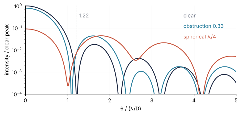
Radial intensity profiles on a log scale out to 5 λ/D for a clear pupil, a pupil with a central obstruction of 0.33, and λ/4 RMS spherical aberration, relative to the clear peak. The obstruction narrows the core and brightens the rings; the aberration lowers the peak and fills the dark rings.

The obstruction keeps 0.793 of the peak and pulls the first dark ring in from 1.220 to 1.097 λ/D. By Rayleigh's measure that is better resolution, and it is not: the light inside the first ring drops from 83.8 % to 65.4 %, and the rest goes into rings that swamp a faint neighbor. Spherical aberration goes after the peak instead. At λ/14 the peak keeps 0.816 and the first minimum moves only to 1.192 λ/D, but it is no longer dark: it holds 0.3 % of the peak. At λ/4 the peak falls to 0.090, the minimum slides in to 1.012 λ/D, and the rings melt into a halo; Hubble's primary mirror went up in 1990 with this aberration. Rayleigh's number assumes a perfect lens, and an imperfect one loses contrast long before it loses its first ring.

Formalization

The sum of phasors, written for a pupil in two dimensions, is the Fraunhofer diffraction integral. The field in the direction \((\theta_x, \theta_y)\) and the PSF are

\[U(\theta_x, \theta_y) \propto \iint P(x, y)\, e^{-2\pi i (x\theta_x + y\theta_y)/\lambda}\, dx\, dy, \qquad I = |U|^2 ,\]

with \(P\) the pupil function: 1 inside the aperture and 0 outside, times \(e^{2\pi i W/\lambda}\) where there is a wavefront error \(W\). The integral is the two-dimensional Fourier transform of the pupil at the spatial frequency \(\theta/\lambda\), the transform that the MRI k-space tutorial takes with fft2. Integrating over \(y\) first leaves the chord length as the weight of each \(x\): the chord-weighted probe above. For a circle of diameter \(D\) the integral is the Airy pattern

\[I(\theta) = I_0 \left[\frac{2 J_1(v)}{v}\right]^2, \qquad v = \frac{\pi D \theta}{\lambda},\]

with \(I_0\) the peak and \(J_1\) the Bessel function of the first kind of order one, scipy.special.j1.

Sample the pupil with \(d\) samples across its diameter, set it in an \(N \times N\) grid of zeros, and the 2D DFT, centered with ifftshift and fftshift, samples \(U\). Index \(k\) of the result is the angle

\[\theta_k = \frac{k\,\lambda}{N \Delta x} = \frac{k}{Q}\,\frac{\lambda}{D}, \qquad \Delta x = \frac{D}{d}, \quad Q = \frac{N}{d} ,\]

so \(Q\) counts samples per \(\lambda/D\). The zeros add no information, only finer sampling: the zero-filling of the MRI tutorial. With \(d = 128\) and \(N = 1024\), \(Q = 8\), and the first dark ring falls at index 9.76, between samples. In the sample plane of a microscope \(\lambda/D\) becomes \(\lambda/(2\,\mathrm{NA})\), as the next paragraph shows, so one sample is 520 nm / (2 × 1.4 × 8) = 23.2 nm.

The first dark ring. The first zero of \(J_1\) is at \(v = 3.8317\), so the first dark ring sits at \(\theta = 1.2197\,\lambda/D\). A microscope measures in the sample, and three steps take the angle there. On the camera side a lens of focal length \(f\) turns the angle into a radius,

\[r' = f\theta = 1.22\,\frac{\lambda f}{D} .\]

An objective that images sharply off the axis obeys Abbe's sine condition, which makes the half-width of the beam \(D/2 = f \sin\alpha'\), with \(\alpha'\) the half-angle of the cone arriving at the camera:

\[r' = 0.61\,\frac{\lambda}{\sin\alpha'} .\]

The same condition links the two sides of the objective, \(n \sin\alpha = M \sin\alpha'\) with \(M\) the magnification, so in the sample

\[r = \frac{r'}{M} = 0.61\,\frac{\lambda}{M \sin\alpha'} = 0.61\,\frac{\lambda}{\mathrm{NA}} .\]

For a 100× objective with NA 1.4, \(\sin\alpha' = 0.014\), the ring has a radius of 22.7 µm on the camera and 226.5 nm in the sample. This is the scalar result; at NA 1.4 polarization reshapes the spot a little, but the field still quotes 0.61 λ/NA.

Rayleigh's criterion. Put two Airy patterns one Rayleigh distance apart and add them: the profile between the peaks dips to 73.5 % of the peak height, a dip of 26.5 %. At 0.8 Rayleigh distances the dip is 0.5 %, at 1.2 it is 56.4 %, and it vanishes at 0.777, Sparrow's criterion. Rayleigh's line is a convention about contrast. Use it to compare instruments, never as the distance below which two points cannot be told apart.

The cutoff, which is not a convention. The image is the object convolved with the PSF, as in the convolution tutorial. Under the Fourier transform a convolution becomes a multiplication, so the object's spectrum is multiplied by the transform of the PSF, the optical transfer function (OTF). The PSF is the product \(U U^*\), and the same theorem run backward turns the transform of a product into the convolution of the transforms. \(U\) is the transform of the pupil, by the integral above, so transforming \(U\) back gives the pupil, and \(U^*\) gives the pupil turned by 180° and conjugated. A convolution with a turned copy is the plus-sign sum the convolution tutorial calls correlation. The OTF at a spatial frequency \(\nu\) of the image is therefore the overlap of the pupil with a copy of itself shifted by \(\lambda \nu\): the autocorrelation of the pupil. Two disks of diameter \(D\) stop overlapping at a shift of \(D\), so the OTF is zero beyond \(\nu = D/\lambda\) cycles per radian, which is \(2\,\mathrm{NA}/\lambda\) in the sample. No period finer than \(\lambda/(2\,\mathrm{NA})\) = 185.7 nm reaches the image at any contrast: Abbe's limit. From the sampled PSF, fft2 gives 0.3908 at half the cutoff, against the exact 0.3910, and below \(10^{-15}\) beyond it. Richardson-Lucy deconvolution sharpens an image up to this limit, never past it.

See it in code

The whole computation is one line, np.abs(np.fft.fftshift(np.fft.fft2(np.fft.ifftshift(P))))**2. The cell runs it at three samplings against the j1 formula, then builds the pairs by tilting the pupil: a point off the axis is a plane wave arriving at an angle, which is a linear phase ramp across the pupil.

Show code

for d_, N_ in [(64, 64), (64, 256), (128, 1024)]:
    I = psf((pupil_radius(d_, N_) <= 1).astype(float))
    c = I[N_ // 2, N_ // 2:] / I.max()
    u_k = np.arange(c.size) * d_ / N_                             # angle in λ/D
    near = u_k <= 5
    i = np.argmin(np.abs(u_k - RAYLEIGH))                        # the sample nearest the dark ring
    print(f"d = {d_:4d}  N = {N_:5d}  Q = {N_ / d_:3.0f} per λ/D   largest deviation from j1 "
          f"{np.abs(c[near] - airy(u_k[near])).max():.1e}   nearest the ring: {c[i]:.4f} at {u_k[i]:.3f} λ/D")

kx = (np.arange(N) - N // 2) / d                                 # pupil x in units of D
row = I_clear[N // 2] / I_clear.max()
u_row = (np.arange(N) - N // 2) / Q                               # focal-plane angle in λ/D

def pair(s):
    """Row through two points s λ/D apart, each a tilted pupil, intensities added."""
    total = 0
    for shift in (-s / 2, s / 2):
        total = total + psf(disk * np.exp(2j * np.pi * kx * shift))
    return total / I_clear.max()

def dip_of(r):
    j = np.argmax(r)                                              # the peak lies between samples:
    top = r[j] + (r[j - 1] - r[j + 1])**2 / (8 * (2 * r[j] - r[j - 1] - r[j + 1]))   # parabola through three
    return 1 - r[N // 2] / top

pairs = {m: pair(m * RAYLEIGH) for m in [0.8, 1.0, 1.2]}
half = round(RAYLEIGH / 2 * Q)                                    # half the separation in whole samples
rolled = np.roll(row, half) + np.roll(row, -half)
print(f"Rayleigh pair: phase ramp dip {100 * dip_of(pairs[1.0][N // 2]):.1f} %, "
      f"np.roll by {half} samples dip {100 * dip_of(rolled):.1f} %")

fig = plt.figure(figsize=(8, 7.4), layout="constrained")
fig.get_layout_engine().set(wspace=0.1)
top, bottom = fig.subfigures(2, 1, height_ratios=[1, 1.25])
ax_pupil, ax_psf, ax_cut = top.subplots(1, 3)
w = slice(N // 2 - int(0.75 * d), N // 2 + int(0.75 * d))
ax_pupil.imshow(disk[w, w], cmap=ListedColormap(["white", INK]), extent=(-0.75, 0.75, -0.75, 0.75))
ax_pupil.set(xlabel="x / D", ylabel="y / D")
ax_pupil.grid(False)
f5 = slice(N // 2 - int(5 * Q), N // 2 + int(5 * Q) + 1)
im = ax_psf.imshow(I_clear[f5, f5] / I_clear.max(), cmap="cividis", norm=LogNorm(1e-4, 1), extent=(-5, 5, -5, 5))
ax_psf.set(xlabel="θx / (λ/D)", ylabel="θy / (λ/D)")
ax_psf.grid(False)
top.colorbar(im, ax=ax_psf, shrink=0.8, aspect=15, ticks=[1e-4, 1e-2, 1], label="intensity / peak")
fine = np.linspace(0, 5, 1000)
ax_cut.semilogy(fine, airy(fine), color=INK, lw=1.2)
ax_cut.semilogy(u_row[N // 2:N // 2 + int(5 * Q) + 1], row[N // 2:N // 2 + int(5 * Q) + 1], "o", ms=4, color=ACCENT)
ax_cut.axvline(RAYLEIGH, color=MUTED, ls="--", lw=1)
ax_cut.set(xlabel="θ / (λ/D)", ylabel="intensity / peak", ylim=(1e-4, 1.5), xlim=(0, 5))

s3 = slice(N // 2 - int(2.5 * Q), N // 2 + int(2.5 * Q) + 1)
s1 = slice(N // 2 - 11, N // 2 + 12)                              # ±11 samples, 1.375 λ/D
grid = bottom.add_gridspec(2, 3, height_ratios=[0.5, 1])
for col, m in enumerate([0.8, 1.0, 1.2]):
    s = m * RAYLEIGH
    image = sum(psf(disk * np.exp(2j * np.pi * kx * sh)) for sh in (-s / 2, s / 2)) / I_clear.max()
    ax_img = bottom.add_subplot(grid[0, col])
    ax_img.imshow(image[s1, s3], cmap="cividis", vmin=0, vmax=1.3, extent=(-2.5, 2.5, -11 / Q, 11 / Q), aspect="auto")
    ax_img.set_axis_off()
    ax_p = bottom.add_subplot(grid[1, col])
    ax_p.plot(u_row[s3], airy(u_row[s3] - s / 2), color=MUTED, lw=1)
    ax_p.plot(u_row[s3], airy(u_row[s3] + s / 2), color=MUTED, lw=1)
    ax_p.plot(u_row[s3], pairs[m][N // 2][s3], color=ACCENT)
    ax_p.text(0, 1.57, f"{m:.1f} Rayleigh", ha="center", va="top", color=INK)
    ax_p.text(0, 1.38, f"dip {100 * dip_of(pairs[m][N // 2]):.1f} %", ha="center", va="top", color=ACCENT)
    ax_p.set(xlabel="θ / (λ/D)", xlim=(-2.5, 2.5), ylim=(0, 1.6))
    if col == 0:
        ax_p.set_ylabel("intensity / peak")
plt.show()

d =   64  N =    64  Q =   1 per λ/D   largest deviation from j1 5.8e-04   nearest the ring: 0.0329 at 1.000 λ/D
d =   64  N =   256  Q =   4 per λ/D   largest deviation from j1 8.7e-04   nearest the ring: 0.0004 at 1.250 λ/D
d =  128  N =  1024  Q =   8 per λ/D   largest deviation from j1 4.0e-04   nearest the ring: 0.0004 at 1.250 λ/D
Rayleigh pair: phase ramp dip 26.4 %, np.roll by 5 samples dip 30.4 %

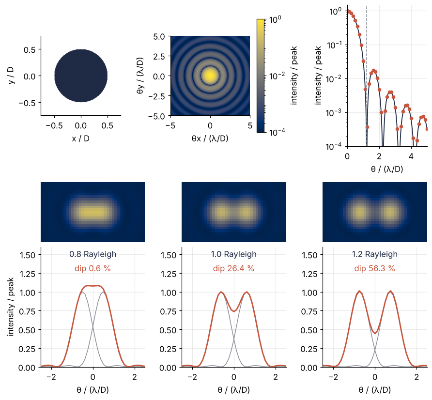
With 128 samples across the pupil and \(Q = 8\) the FFT agrees with the Bessel formula to 4.0 × 10⁻⁴ of the peak, and the residual comes from the stair-step edge of the sampled disk. Without padding, \(Q = 1\), there is one sample per \(\lambda/D\). The sample nearest the dark ring sits at 1.0 λ/D with 3.3 % of the peak, and the pattern is a blocky dot with no ring in it. The phase ramp shifts the pattern by any fraction of a sample, and the bottom row agrees with the Formalization's exact dips to within 0.1 percentage point, the size of the stair-step error. Rolling the array by whole samples puts the Rayleigh pair 1.25 λ/D apart instead of 1.22, and the dip comes out at 30.4 % against the phase ramp's 26.4 %. Shift a PSF with a phase ramp; np.roll is right only when the shift is a whole number of samples.

Where it shows up

Fluorescence microscopy. The limit is about separating two spots, not about locating one, so PALM and STORM switch the molecules on one at a time and find each center far more precisely than 227 nm. STED takes the other route and shrinks the effective PSF itself, switching off the fluorescence everywhere but in the center of the spot.
Telescopes and adaptive optics. From the ground, atmospheric seeing of about 1″ smears the 0.016″ diffraction limit of an 8 m mirror at 500 nm. Adaptive optics measures the wavefront error with a sensor and cancels it with a deformable mirror, which brings back the Airy core of the section on aberrations.
Lithography of microchips. The industry writes Rayleigh's formula for the critical dimension, the smallest printable feature, as CD = k₁ λ/NA, with k₁ a process factor that mask and illumination tricks push toward its floor of 0.25. A 193 nm immersion scanner at NA 1.35 reaches 35.7 nm at that floor, and EUV machines go to a wavelength of 13.5 nm instead.
Cameras and pixel size. The Airy disk on a sensor is 2.44 λN across for f-number N, 10.7 µm at f/8 in green light at 550 nm, wider than two 4 µm pixels. On such a sensor, stopping down further blurs the picture instead of sharpening it.
Radio interferometers. The longest baseline B between two dishes takes the place of D, and the resolution is about λ/B. The Event Horizon Telescope observes at 1.3 mm on baselines up to the diameter of the Earth, which gives λ/B = 21 µas, enough to resolve the ring of Ray tracing a black hole with solve_ivp: the shadow of M87*.

In every case the first number to compute is the aperture in wavelengths, D/λ or B/λ: it sets the finest period the instrument passes at all.

The question

The idea: the lens adds up the waves that cross its aperture

A hole in the pupil and a bent wavefront

Formalization

See it in code

Where it shows up

Further reading