Zernike polynomials in NumPy: a telescope's wavefront and Strehl ratio

The problem: what is wrong with this telescope, and how much does it cost?

A wavefront sensor behind a 200 mm telescope reports, at 316 points over the round pupil, how far the incoming wavefront departs from a perfect one, in nm. It is a Shack-Hartmann sensor, a grid of small lenses every 10 mm that measure the local slope, and its software reconstructs from those slopes the wavefront values we start from. They span 792 nm from the lowest point to the highest, more than the 550 nm wavelength of the green light the telescope is used at.

The standard way to read such a map is a fit with Zernike polynomials, polynomials on the unit disk that are orthogonal to each other and whose first terms are the aberrations an optician names: tilt, defocus, astigmatism, coma, spherical aberration. Their coefficients are the report of an optical test bench, what adaptive optics corrects, and the printout of an eye doctor's aberrometer.

What the aberrations cost has a number: the Strehl ratio \(S\), the peak of the point spread function (PSF), which is the image of a star, divided by the peak a perfect telescope of the same size would give. Maréchal's approximation gets it from the RMS (root mean square) wavefront error \(\sigma\) alone, here in the exponential form that Mahajan showed in 1983 to approximate \(S\) better than the original,

\[S \approx \exp\left[-\left(2\pi\sigma/\lambda\right)^2\right],\]

with \(\lambda\) the wavelength. An error of \(\sigma = \lambda/14\) gives \(S = 0.82\), the usual line for "diffraction-limited". How far can you trust the shortcut, compared with the PSF itself?

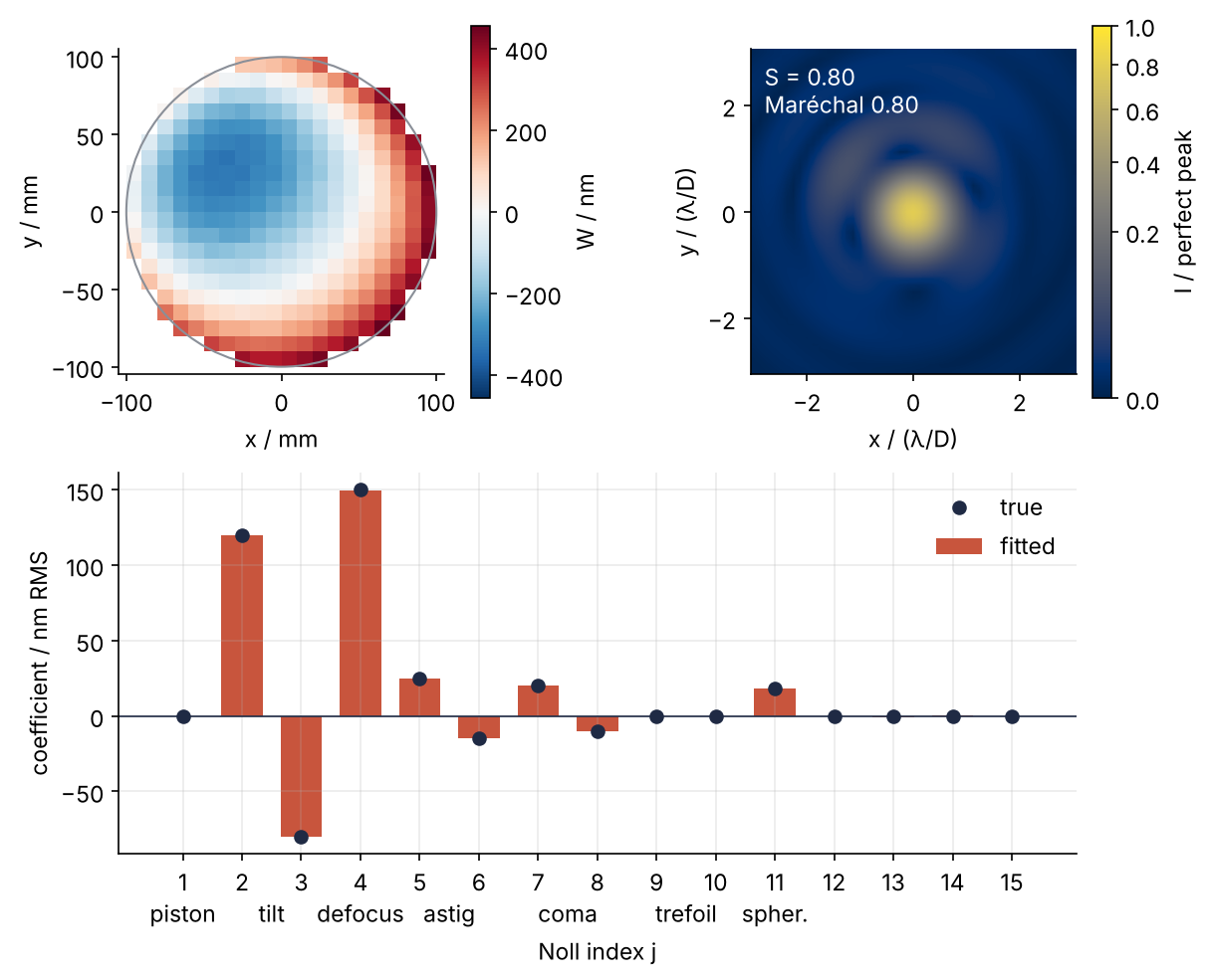
Top left: measured wavefront at 316 points of a 200 mm pupil, in nm, a tilted bowl. Top right: point spread function after removing tilt and defocus, on a square-root color scale, Strehl ratio 0.80. Bottom: the 15 fitted Zernike coefficients as bars on the true values.

Top left is the measurement, at the bottom the 15 fitted coefficients on the true ones, top right the PSF once the mount has taken out the tilt and the focuser the defocus. Its Strehl ratio is 0.80 by Maréchal and from the PSF alike, just short of the line. Step 6 draws the figure.

Setup

The measurement is synthetic, with known aberrations, so that every fitted number can be checked against the truth. The cell lays out the sensor's subaperture centers in mm and converts them to the unit disk. Zernike polynomials and their normalization are defined on the disk of radius 1, so positions from your own sensor, in mm or in pixels, are measured from the pupil center and divided by the pupil radius first. A fit in raw mm gives coefficients that mean nothing.

import numpy as np
import matplotlib.pyplot as plt
from matplotlib.colors import PowerNorm
from math import factorial

plt.rcParams.update({
    "figure.figsize": (7, 3.6), "figure.dpi": 110,
    "axes.spines.top": False, "axes.spines.right": False,
    "axes.grid": True, "grid.alpha": 0.25,
    "font.size": 11, "lines.linewidth": 1.8,
})
INK, ACCENT, SECOND, MUTED = "#1f2a44", "#c8553d", "#2a7f9e", "#8a8f98"

rng = np.random.default_rng(282)           # Step 3 draws the sensor noise from it
wavelength = 550.0                         # nm
noise_rms = 5.0                            # nm per sensor point

# subaperture centers every 10 mm; the pupil has its center at (x0, y0) and radius R
grid_mm = np.arange(-95.0, 96.0, 10.0)
x_mm, y_mm = [a.ravel() for a in np.meshgrid(grid_mm, grid_mm)]
x0, y0, R = 0.0, 0.0, 100.0                # mm
r_mm = np.hypot(x_mm - x0, y_mm - y0)
inside = r_mm <= R
x_mm, y_mm = x_mm[inside], y_mm[inside]
rho = r_mm[inside] / R                     # the unit disk the polynomials live on
theta = np.arctan2(y_mm - y0, x_mm - x0)
M = rho.size

c_true = {2: 120, 3: -80, 4: 150, 5: 25, 6: -15, 7: 20, 8: -10, 11: 18}   # Noll j: nm RMS

print(f"{M} sensor points, largest rho = {rho.max():.4f}")

316 sensor points, largest rho = 0.9925

Step 1: Write the Zernike polynomials with Noll indices

Each Zernike polynomial is a radial polynomial times an angular harmonic. With \(n\) the radial order and \(m\) the angular frequency, integers with \(n - |m|\) even and not negative, the polynomial is \(N R_n^{|m|}(\rho)\cos(m\theta)\) for \(m \ge 0\) and \(N R_n^{|m|}(\rho)\sin(|m|\theta)\) for \(m < 0\). The radial part is a finite sum,

\[R_n^{m}(\rho) = \sum_{k=0}^{(n-m)/2} \frac{(-1)^k\,(n-k)!}{k!\,\left(\frac{n+m}{2}-k\right)!\,\left(\frac{n-m}{2}-k\right)!}\,\rho^{\,n-2k},\]

and the factor \(N\) is \(\sqrt{n+1}\) for \(m = 0\) and \(\sqrt{2(n+1)}\) otherwise. It makes the RMS of every polynomial over the disk equal to 1, and that is what you will use every time: a coefficient of 25 nm means the term adds 25 nm RMS to the wavefront.

Noll (1976) numbered the pairs with one index \(j\), ordered by \(n\), then by \(|m|\). Each \(|m| > 0\) comes twice, and the even \(j\) of the pair takes the cosine (\(m > 0\)), the odd \(j\) the sine (\(m < 0\)).

def noll_to_nm(j):
    n = 0
    while (n + 1) * (n + 2) // 2 < j:      # row n holds j up to (n+1)(n+2)/2
        n += 1
    k = j - n * (n + 1) // 2 - 1           # position within the row, 0 to n
    m = 2 * ((k + 1) // 2) if n % 2 == 0 else 2 * (k // 2) + 1
    return (n, -m) if (m != 0 and j % 2 == 1) else (n, m)

def radial(n, m, rho):
    m = abs(m)
    return sum((-1)**k * factorial(n - k)
               / (factorial(k) * factorial((n + m) // 2 - k) * factorial((n - m) // 2 - k))
               * rho**(n - 2 * k) for k in range((n - m) // 2 + 1))

def zernike(j, rho, theta):
    n, m = noll_to_nm(j)
    if m == 0:
        return np.sqrt(n + 1) * radial(n, 0, rho)
    harmonic = np.cos(m * theta) if m > 0 else np.sin(-m * theta)
    return np.sqrt(2 * (n + 1)) * radial(n, m, rho) * harmonic

names = ["piston", "tilt x", "tilt y", "defocus", "oblique astigmatism", "vertical astigmatism",
         "vertical coma", "horizontal coma", "vertical trefoil", "oblique trefoil",
         "primary spherical", "secondary astigmatism", "secondary astigmatism",
         "quadrafoil", "quadrafoil"]
for j in range(1, 12):
    n, m = noll_to_nm(j)
    print(f"j = {j:2d}   (n, m) = ({n}, {m:2d})   {names[j - 1]}")

error = np.max(np.abs(zernike(4, rho, theta) - np.sqrt(3) * (2 * rho**2 - 1)))
print(f"defocus against sqrt(3)(2 rho^2 - 1): largest difference {error:.1e}")

j =  1   (n, m) = (0,  0)   piston
j =  2   (n, m) = (1,  1)   tilt x
j =  3   (n, m) = (1, -1)   tilt y
j =  4   (n, m) = (2,  0)   defocus
j =  5   (n, m) = (2, -2)   oblique astigmatism
j =  6   (n, m) = (2,  2)   vertical astigmatism
j =  7   (n, m) = (3, -1)   vertical coma
j =  8   (n, m) = (3,  1)   horizontal coma
j =  9   (n, m) = (3, -3)   vertical trefoil
j = 10   (n, m) = (3,  3)   oblique trefoil
j = 11   (n, m) = (4,  0)   primary spherical
defocus against sqrt(3)(2 rho^2 - 1): largest difference 0.0e+00

Defocus comes out as \(\sqrt 3(2\rho^2-1)\) to the last bit. Maps of all 15 polynomials up to \(n = 4\) make the names concrete, red for positive and blue for negative:

Show code

v = np.linspace(-1, 1, 201)
VX, VY = np.meshgrid(v, v)
r_map, t_map = np.hypot(VX, VY), np.arctan2(VY, VX)
fig = plt.figure(figsize=(8, 8.8))
size, gap = 0.16, 0.03
for j in range(1, 16):
    n, m = noll_to_nm(j)
    col = (m + n) / 2                      # m runs from -n to n in steps of 2
    left = 0.5 - (n + 1) * (size + gap) / 2 + col * (size + gap)
    ax = fig.add_axes([left, 0.98 - (n + 1) * 0.195, size, size])
    img = np.where(r_map <= 1, zernike(j, r_map, t_map), np.nan)
    ax.imshow(img, cmap="RdBu_r", vmin=-3.2, vmax=3.2, origin="lower")
    ax.set_axis_off()
    ax.text(0.5, -0.04, f"{j}\n{names[j - 1].replace('astigmatism', 'astig.')}", transform=ax.transAxes,
            ha="center", va="top", fontsize=10, color=INK, linespacing=1.1)
plt.show()

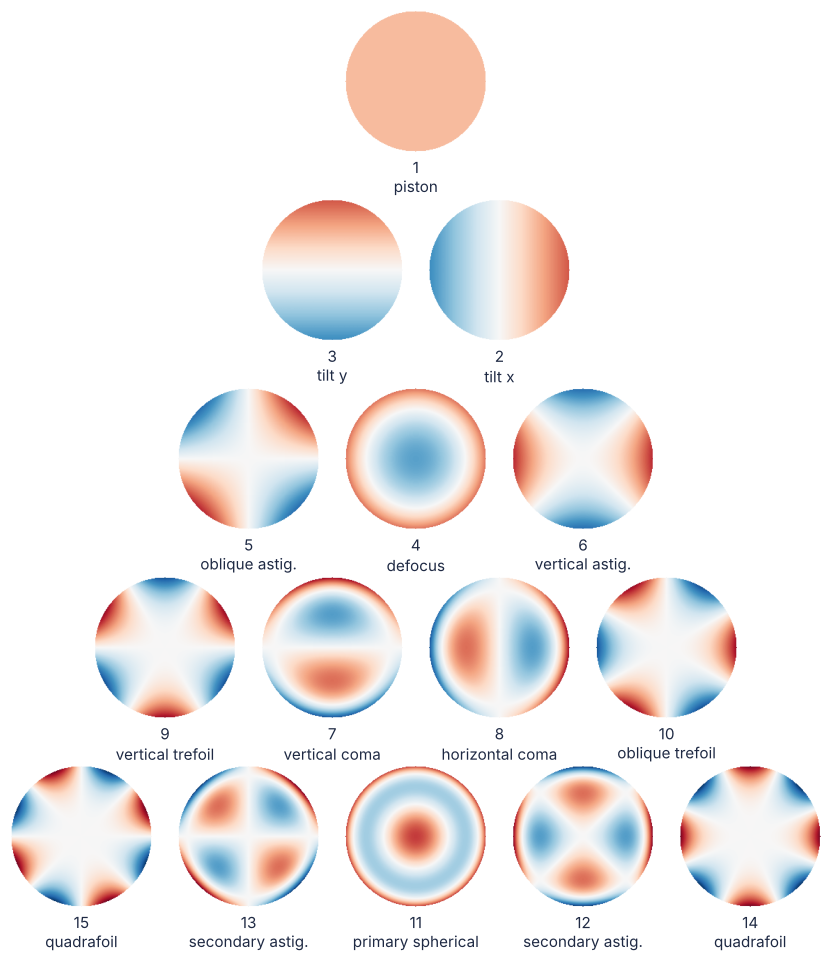
The first 15 Zernike polynomials as maps on the unit disk, one row per radial order n from 0 to 4, red positive and blue negative: piston, the two tilts, defocus, astigmatism, coma, trefoil, and spherical aberration, each labeled with its Noll index.

Tilt is a plane, defocus a bowl, astigmatism a saddle, and coma a tilt that bends back near the rim. Primary spherical aberration is high at the center and at the rim and low in between, a ring-shaped error that no focus setting removes.

Step 2: Check that they are orthogonal on the pupil

Orthogonal means that the average of \(Z_i Z_j\) over the disk is 1 for \(i = j\) and 0 otherwise. Two things follow. Each coefficient could be found on its own as the average of the data times its polynomial, the Fourier-coefficient way. And the RMS of a wavefront over the disk is the square root of the sum of its squared coefficients, which Step 4 uses. Compute the matrix of those averages, the Gram matrix, on a dense 256 × 256 pupil grid and on the 316 sensor points:

Np = 256                                   # pixels across the pupil; Steps 4 and 5 use this grid too
u = (np.arange(Np) + 0.5) / (Np / 2) - 1
UX, UY = np.meshgrid(u, u)
pupil = np.hypot(UX, UY) <= 1
rho_d, theta_d = np.hypot(UX, UY)[pupil], np.arctan2(UY, UX)[pupil]

J = 15
Z_dense = np.column_stack([zernike(j, rho_d, theta_d) for j in range(1, J + 1)])
A = np.column_stack([zernike(j, rho, theta) for j in range(1, J + 1)])

for label, Z in [("dense pupil grid", Z_dense), ("316 sensor points", A)]:
    G = Z.T @ Z / len(Z)
    off = np.abs(G - np.diag(np.diag(G))).max()
    print(f"{label:17s}  diagonal {np.diag(G).min():.3f} to {np.diag(G).max():.3f},"
          f"  largest off-diagonal {off:.3f}")

dense pupil grid   diagonal 0.998 to 1.001,  largest off-diagonal 0.002
316 sensor points  diagonal 0.950 to 1.088,  largest off-diagonal 0.025

On the dense grid the matrix is the identity to within 0.002. On the sensor points the diagonal runs from 0.950 to 1.088 and the off-diagonal entries reach 0.025: the polynomials are orthogonal on the continuous disk, not on a coarse sample of it, so the Fourier-coefficient way would mix the terms a little. Least squares needs no orthogonality, which is why Step 3 uses it. The second pitfall shows a pupil where projection fails badly.

Step 3: Fit the measured wavefront by least squares

The measurement is the true wavefront at the sensor points plus 5 nm of noise per point. Its RMS and its PV (peak to valley, the highest value minus the lowest) are the two numbers a test report starts with:

c_vec = np.zeros(J)
for j, value in c_true.items():
    c_vec[j - 1] = value
W = A @ c_vec + rng.normal(0, noise_rms, M)
print(f"measured wavefront: RMS {np.sqrt(np.mean(W**2)):.0f} nm, PV {np.ptp(W):.0f} nm")

measured wavefront: RMS 213 nm, PV 792 nm

The model is linear in the coefficients, so this is the problem of least squares: the design matrix A from Step 2 has one column per polynomial, 316 rows by 15 columns, and your own data enters here as rho and theta after the conversion of Setup. The fitted coefficients are a fixed linear map of the data, \(c = (A^\mathsf{T}A)^{-1}A^\mathsf{T}W\). A linear map \(B\) turns independent noise of variance \(s^2\) into the covariance matrix \(s^2BB^\mathsf{T}\), which for this \(B\) is \(s^2(A^\mathsf{T}A)^{-1}\), and the square roots of its diagonal are the standard errors. It is the matrix curve_fit returns as pcov when you give it sigma and absolute_sigma=True.

c_fit, *_ = np.linalg.lstsq(A, W, rcond=None)
cov = noise_rms**2 * np.linalg.inv(A.T @ A)
se = np.sqrt(np.diag(cov))

print(" j   fitted / nm      true / nm")
for j in range(1, J + 1):
    print(f"{j:2d}  {c_fit[j - 1]:7.2f} ± {se[j - 1]:.2f}   {c_vec[j - 1]:6.0f}")
print(f"largest |fitted - true| = {np.max(np.abs(c_fit - c_vec)):.2f} nm,"
      f"  residual RMS = {np.sqrt(np.mean((W - A @ c_fit)**2)):.2f} nm")

 j   fitted / nm      true / nm
 1    -0.32 ± 0.28        0
 2   120.08 ± 0.28      120
 3   -79.77 ± 0.28      -80
 4   149.50 ± 0.28      150
 5    25.04 ± 0.28       25
 6   -15.04 ± 0.28      -15
 7    20.36 ± 0.28       20
 8    -9.84 ± 0.28      -10
 9    -0.06 ± 0.28        0
10     0.08 ± 0.28        0
11    17.92 ± 0.28       18
12    -0.45 ± 0.28        0
13    -0.84 ± 0.28        0
14     0.12 ± 0.27        0
15    -0.15 ± 0.29        0
largest |fitted - true| = 0.84 nm,  residual RMS = 4.91 nm

Every coefficient lands within about three standard errors of the truth, the largest miss is 0.84 nm on a standard error of 0.28 nm, and the terms that are zero come out below 1 nm. The residual RMS is 4.91 nm, the 5 nm noise and nothing more, so 15 terms describe this wavefront completely.

Step 4: Remove tilt and defocus and estimate the Strehl ratio

The \(\sigma\) in Maréchal's formula is the RMS of the fitted wavefront over the full continuous disk, the function the coefficients describe, not over the 316 samples. By the orthogonality of Step 2 it is \(\sqrt{\sum c_j^2}\). Piston is left out, because a constant phase changes nothing in the image. Tilt only moves the image sideways: a phase that grows linearly across the pupil shifts the pattern in the focal plane without changing its shape, and the mount corrects it. Defocus is what the focuser corrects.

sigma_tilt = np.sqrt(np.sum(c_fit[3:]**2))         # without piston and tilt, j = 1 to 3
sigma_res = np.sqrt(np.sum(c_fit[4:]**2))          # without defocus, j = 4, too
c_res = c_fit.copy()
c_res[:4] = 0
rms_dense = np.sqrt(np.mean((Z_dense @ c_res)**2))

print(f"tilt removed:            sigma = {sigma_tilt:6.1f} nm = lambda/{wavelength / sigma_tilt:.1f}")
print(f"tilt and defocus removed: sigma = {sigma_res:6.1f} nm = lambda/{wavelength / sigma_res:.1f}")
print(f"RMS of that residual on the dense pupil grid: {rms_dense:.1f} nm")
print(f"Maréchal: residual S = {np.exp(-(2 * np.pi * sigma_res / wavelength)**2):.3f},"
      f"  at lambda/14 S = {np.exp(-(2 * np.pi / 14)**2):.3f}")
for j in range(5, J + 1):
    if c_res[j - 1]**2 / sigma_res**2 > 0.01:
        print(f"  j = {j:2d} {names[j - 1]:22s} {100 * c_res[j - 1]**2 / sigma_res**2:4.1f} % of the variance")

tilt removed:            sigma =  155.0 nm = lambda/3.5
tilt and defocus removed: sigma =   41.1 nm = lambda/13.4
RMS of that residual on the dense pupil grid: 41.1 nm
Maréchal: residual S = 0.802,  at lambda/14 S = 0.818
  j =  5 oblique astigmatism    37.2 % of the variance
  j =  6 vertical astigmatism   13.4 % of the variance
  j =  7 vertical coma          24.6 % of the variance
  j =  8 horizontal coma         5.7 % of the variance
  j = 11 primary spherical      19.0 % of the variance

Focusing takes the error from \(\lambda/3.5\) to \(\lambda/13.4\), and the dense grid confirms the 41.1 nm. Maréchal gives the residual \(S = 0.802\), just short of the 0.818 at \(\lambda/14\). The coefficients say which term to fix next: the two astigmatisms carry half the variance that is left, the oblique one 37.2 % alone. The defocused wavefront gets no Maréchal number here, because the formula is an approximation for small errors and \(\lambda/3.5\) is far from small. Step 5 measures both.

Step 5: Compute the point spread function and its Strehl ratio

In the focal plane of a telescope the light field is the two-dimensional Fourier transform of the field in the pupil, \(P\exp(2\pi i W/\lambda)\), where \(P\) is 1 inside the pupil and \(2\pi W/\lambda\) is the phase that the path difference \(W\) adds. This tutorial uses the result without deriving it; the angular spectrum tutorial and Goodman (Further reading) derive it. The PSF is the squared modulus of that transform, computed with np.fft.fft2 (the Fourier transform tutorial has the background). Its natural angular unit is \(\lambda/D\), with \(D\) the pupil diameter: the perfect PSF has its first dark ring at \(1.22\,\lambda/D\).

The spacing of a discrete transform's frequencies is one over the length of the array. The pupil fills its 256 samples, so the unpadded transform gives one sample per \(\lambda/D\), and padding the 256 × 256 pupil with zeros to 2048 × 2048 samples the same PSF eight times more finely, 8 points per \(\lambda/D\), and the peak is not missed between samples. fft2 pads for you when you give it the output size s. The Strehl ratio is the ratio of two peaks computed the same way, so no normalization constant matters.

pad = 8 * Np

def psf(coeffs):
    W_pupil = np.zeros((Np, Np))
    W_pupil[pupil] = Z_dense @ coeffs
    field = pupil * np.exp(2j * np.pi * W_pupil / wavelength)
    return np.abs(np.fft.fft2(field, s=(pad, pad)))**2

peak_perfect = psf(np.zeros(J)).max()
strehl = lambda coeffs: psf(coeffs).max() / peak_perfect
marechal = lambda sigma: np.exp(-(2 * np.pi * sigma / wavelength)**2)

c_defocus = c_fit.copy()
c_defocus[:3] = 0                          # tilt removed, defocus kept
for label, coeffs, sigma in [("tilt and defocus removed", c_res, sigma_res),
                             ("defocus kept", c_defocus, sigma_tilt)]:
    print(f"{label:24s}  S from PSF {strehl(coeffs):.4f}   Maréchal {marechal(sigma):.4f}")

tilt and defocus removed  S from PSF 0.8025   Maréchal 0.8025
defocus kept              S from PSF 0.1083   Maréchal 0.0434

For the residual the two agree to four digits. With defocus kept, the PSF gives 0.108 and Maréchal 0.043. To see where they part, scale the residual by factors from 0.5 to 4:

factors = np.arange(0.5, 4.01, 0.5)
s_wave = factors * sigma_res / wavelength
S_direct = np.array([strehl(f * c_res) for f in factors])
for s, S in zip(s_wave, S_direct):
    print(f"sigma = {s:.3f} waves   PSF {S:.3f}   Maréchal {marechal(s * wavelength):.3f}")

s_line = np.linspace(0, 0.31, 200)
fig, ax = plt.subplots()
ax.plot(s_line, marechal(s_line * wavelength), color=INK, label="Maréchal")
ax.plot(s_wave, S_direct, "o", color=ACCENT, ms=6, label="peak of the PSF")
ax.plot(sigma_tilt / wavelength, strehl(c_defocus), "o", ms=6, mfc="none", mec=ACCENT)
ax.annotate("defocus kept", (sigma_tilt / wavelength, strehl(c_defocus) + 0.02), (0.282, 0.33),
            color=ACCENT, ha="center", arrowprops=dict(arrowstyle="-", color=ACCENT, lw=1))
S_line = marechal(wavelength / 14)
ax.axvline(1 / 14, color=MUTED, lw=1, ls="--")
ax.axhline(S_line, color=MUTED, lw=1, ls="--")
ax.text(1 / 14 + 0.004, 0.03, "λ/14", color=MUTED)
ax.text(0.308, S_line + 0.02, f"S = {S_line:.2f}", color=MUTED, ha="right", va="bottom")
ax.set(xlabel="σ / λ", ylabel="Strehl ratio S", xlim=(0, 0.31), ylim=(0, 1.02))
ax.legend(frameon=False, loc="upper right", bbox_to_anchor=(1, 0.74))
plt.show()

sigma = 0.037 waves   PSF 0.946   Maréchal 0.946
sigma = 0.075 waves   PSF 0.802   Maréchal 0.802
sigma = 0.112 waves   PSF 0.609   Maréchal 0.609
sigma = 0.149 waves   PSF 0.421   Maréchal 0.415
sigma = 0.187 waves   PSF 0.271   Maréchal 0.253
sigma = 0.224 waves   PSF 0.186   Maréchal 0.138
sigma = 0.261 waves   PSF 0.165   Maréchal 0.067
sigma = 0.299 waves   PSF 0.137   Maréchal 0.030

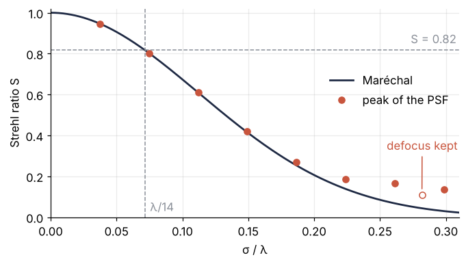
Strehl ratio against RMS wavefront error in waves, from 0 to 0.3. Line: Maréchal approximation. Dots: peak ratio of the computed PSF. They agree below about 0.15 waves; above it Maréchal falls lower, and the defocused wavefront at 0.28 waves sits far above the line.

The two agree to within 0.006 up to \(\sigma = 0.149\lambda\), about \(\lambda/7\), and part beyond it, Maréchal always lower: at \(0.299\lambda\) the PSF gives 0.137 and Maréchal 0.030. The defocused wavefront lies far into that region, so Maréchal's 0.043 says only that the image is bad. What focusing really gains is the PSF's factor, from 0.108 to 0.802.

Step 6: Draw the wavefront, the coefficients, and the PSF

The signed wavefront gets a diverging colormap, RdBu_r, centered on zero; the PSF gets cividis on a square-root scale, so that the faint ring shows, divided by the perfect peak so that its color bar reads the Strehl ratio. fft2 puts the zero angle, the center of the PSF, at index [0, 0] and wraps the negative angles to the far end of the array. np.fft.fftshift moves it to the middle, index pad // 2, and the crop keeps ±3 \(\lambda/D\) around it.

fig = plt.figure(figsize=(8, 6.6), layout="constrained")
gs = fig.add_gridspec(2, 2, height_ratios=[1.15, 1])

ax = fig.add_subplot(gs[0, 0])
vmax = np.abs(W).max()
W_map = np.full((grid_mm.size, grid_mm.size), np.nan)    # the 10 mm sensor grid as an image
W_map[np.searchsorted(grid_mm, y_mm), np.searchsorted(grid_mm, x_mm)] = W
im = ax.imshow(W_map, cmap="RdBu_r", vmin=-vmax, vmax=vmax, origin="lower",
               extent=[-100, 100, -100, 100])
ax.add_patch(plt.Circle((x0, y0), R, fill=False, color=MUTED, lw=1))
ax.set(xlabel="x / mm", ylabel="y / mm", xlim=(-105, 105), ylim=(-105, 105))
ax.grid(False)
fig.colorbar(im, ax=ax, label="W / nm", shrink=0.85)
fig.get_layout_engine().set(wspace=0.12)

ax = fig.add_subplot(gs[0, 1])
half = 24                                  # ±3 λ/D at 8 samples per λ/D
I = np.fft.fftshift(psf(c_res)) / peak_perfect
crop = I[pad // 2 - half:pad // 2 + half + 1, pad // 2 - half:pad // 2 + half + 1]
im = ax.imshow(crop, cmap="cividis", norm=PowerNorm(0.5, vmin=0, vmax=1),   # square root: the faint ring shows
               origin="lower", interpolation="bilinear",
               extent=[-half / 8 - 1 / 16, half / 8 + 1 / 16] * 2)   # outer pixel edges, half a sample out
ax.text(-2.8, 2.8, f"S = {strehl(c_res):.2f}\nMaréchal {marechal(sigma_res):.2f}",
        color="white", va="top")
ax.set(xlabel="x / (λ/D)", ylabel="y / (λ/D)", xticks=[-2, 0, 2], yticks=[-2, 0, 2])
ax.grid(False)
fig.colorbar(im, ax=ax, label="I / perfect peak", shrink=0.85)

ax = fig.add_subplot(gs[1, :])
j_all = np.arange(1, J + 1)
ax.bar(j_all, c_fit, color=ACCENT, width=0.7, label="fitted")
ax.plot(j_all, c_vec, "o", color=INK, ms=6, label="true")
ax.axhline(0, color=INK, lw=0.8)
ax.set_xticks(j_all)
for j, name in [(1, "piston"), (2.5, "tilt"), (4, "defocus"), (5.5, "astig"), (7.5, "coma"),
                (9.5, "trefoil"), (11, "spher.")]:    # one name under each pair of j
    ax.text(j, -0.12, name, transform=ax.get_xaxis_transform(), ha="center", va="top")
ax.set_xlabel("Noll index j", labelpad=20)
ax.set_ylabel("coefficient / nm RMS")
ax.legend(frameon=False, loc="upper right")
plt.show()

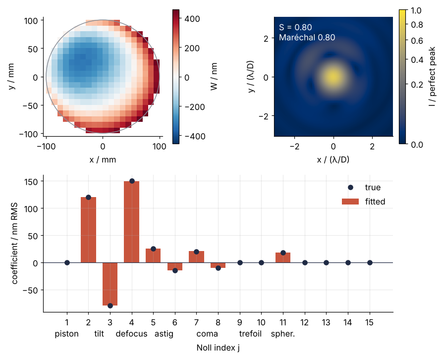
Top left: measured wavefront at 316 points of a 200 mm pupil, in nm, a tilted bowl. Top right: point spread function after removing tilt and defocus, on a square-root color scale, Strehl ratio 0.80. Bottom: the 15 fitted Zernike coefficients as bars on the true values.

The measured wavefront is a bowl tilted toward the lower right. The fitted bars sit on the true markers at every index. The PSF of the residual is a bright core with a first ring all the way around, brightest on the upper left, lopsided by the astigmatism and coma that remain.

Pitfalls

Index conventions. Coefficients from an instrument or a paper do not match yours, or spherical aberration turns up as "Z9" or "Z12". Three orderings are in use: Noll in astronomy, as here; OSA/ANSI in ophthalmology, which starts at \(j = 0\) and sets \(j = (n(n+2) + m)/2\); and Fringe in lens design software, which numbers spherical aberration 9 in its published table and often leaves the polynomials unnormalized, with value 1 at the rim instead of RMS 1.

def nm_to_osa(n, m):
    return (n * (n + 2) + m) // 2

for j in [4, 5, 6, 11]:
    n, m = noll_to_nm(j)
    print(f"{names[j - 1]:20s} (n, m) = ({n}, {m:2d})   Noll {j:2d}   OSA/ANSI {nm_to_osa(n, m):2d}")

defocus              (n, m) = (2,  0)   Noll  4   OSA/ANSI  4
oblique astigmatism  (n, m) = (2, -2)   Noll  5   OSA/ANSI  3
vertical astigmatism (n, m) = (2,  2)   Noll  6   OSA/ANSI  5
primary spherical    (n, m) = (4,  0)   Noll 11   OSA/ANSI 12

Convert every index to \((n, m)\) and every coefficient to the RMS normalization before you compare. Fringe coefficients must be rescaled before they go into Maréchal's formula.

Orthogonality on a pupil with a hole. Coefficients obtained by projection, the average of the data times each polynomial, come out wrong, spherical aberration most of all. The polynomials are orthogonal on the full disk only, and the secondary mirror of a reflecting telescope blocks the center. Here the obstruction ratio, the blocked radius over the pupil radius, is 0.35, in the range of Cassegrain telescopes:

keep = rho >= 0.35
A_ring, W_ring = A[keep], W[keep]
G = A_ring.T @ A_ring / keep.sum()
off = np.abs(G - np.diag(np.diag(G)))
i, k = np.unravel_index(off.argmax(), off.shape)
c_proj = A_ring.T @ W_ring / keep.sum()
c_lsq, *_ = np.linalg.lstsq(A_ring, W_ring, rcond=None)
print(f"{keep.sum()} points left; largest off-diagonal {off.max():.2f}, between j = {i + 1} and j = {k + 1}")
print(f"spherical (j = 11): projection {c_proj[10]:.1f} nm, lstsq {c_lsq[10]:.1f} nm, true 18 nm")

284 points left; largest off-diagonal 0.30, between j = 4 and j = 11
spherical (j = 11): projection 60.2 nm, lstsq 18.0 nm, true 18 nm

The average of \(Z_4 Z_{11}\) over the ring is now 0.30 instead of 0, so defocus and spherical aberration are no longer independent, and projection credits spherical with 60.2 nm, more than three times its true 18 nm. Always fit with lstsq, which needs no orthogonality; for a heavy obstruction there is an annular basis (Variations).

Waves against nanometers. A Strehl ratio of 0 or 1 to three digits, or a mirror that is diffraction-limited in its test report and not on the sky. Either \(\sigma\) and \(\lambda\) are in different units, or \(\sigma\) was quoted in waves of the test wavelength, often the 633 nm of a helium-neon interferometer, and used at another. The same 41.1 nm residual is \(\lambda/15.4\) with \(S = 0.847\) at 633 nm, but \(\lambda/13.4\) with \(S = 0.802\) at 550 nm, on the wrong side of the line. Keep the wavefront in nm and divide by the wavelength of use only inside the formula.

Variations

More terms. Fit \(j\) up to 36 by changing J. The condition number np.linalg.cond(A), the largest singular value of A over the smallest, is roughly the factor by which the fit can amplify relative errors in the data, 1 for orthonormal columns. At \(J = 36\) it is still 1.38, and the 21 extra coefficients reach 0.73 nm at most, noise. It is 12 at \(J = 105\) and \(8 \times 10^{13}\) at \(J = 231\), where the fit breaks: the product \((x - x_1)\cdots(x - x_{20})\) over the 20 sensor columns is a polynomial of degree 20, so a combination of the 231 polynomials, and it is zero at every sensor point, so no data can fix its coefficient.
An annular pupil. Replace the disk polynomials by Mahajan's annular Zernike polynomials, orthogonal on the ring, with the obstruction ratio as a parameter.
The eye. Use OSA/ANSI indices, a pupil of 6 mm diameter, so \(R = 3\) mm in Setup, and coefficients in µm, the format of an aberrometer report.
Adaptive optics. A deformable mirror corrects the wavefront by adding the fitted terms times \(-1\), which takes a surface of minus half the fitted wavefront at normal incidence, since reflection doubles every path change; subtract the corrected terms from c_res and Step 5 gives the Strehl ratio of the corrected image.

Cheat sheet

rho, theta = np.hypot(x - x0, y - y0) / R, np.arctan2(y - y0, x - x0)   # pupil center (x0, y0), radius R
n, m = noll_to_nm(j)                                     # Noll: even j cosine (m > 0), odd j sine (m < 0)
Z = np.sqrt(2 * (n + 1)) * radial(n, m, rho) * np.cos(m * theta)   # m > 0; sin(|m| θ) for m < 0, sqrt(n + 1) for m = 0
A = np.column_stack([zernike(j, rho, theta) for j in range(1, 16)])
c, *_ = np.linalg.lstsq(A, W, rcond=None)                # coefficients in nm RMS, never by projection
se = np.sqrt(np.diag(s**2 * np.linalg.inv(A.T @ A)))     # standard errors, s the noise per point
sigma = np.sqrt(np.sum(c[4:]**2))                        # RMS without piston, tilt, defocus (j = 1 to 4)
S_marechal = np.exp(-(2 * np.pi * sigma / wavelength)**2)    # sigma and wavelength in the same unit
psf = lambda Wp: np.abs(np.fft.fft2(pupil * np.exp(2j * np.pi * Wp / wavelength), s=(8 * Np, 8 * Np)))**2
S = psf(W_pupil).max() / psf(0 * W_pupil).max()          # Strehl ratio, peak over the perfect peak