Single-diode fit with curve_fit and lambertw: a solar cell's I-V curve (Python)

The problem: five parameters from one I-V curve

Put a crystalline silicon cell, a full-size wafer, under a flash lamp at 25 °C, sweep the voltage, and you get its I-V curve: 60 points from 9.00 A at short circuit down to zero current at 0.651 V. The numbers here are illustrative values typical of such a cell. What you want from the curve are the five parameters of the single-diode model, a current source, a diode, and a shunt resistance in parallel, all behind a series resistance:

\[I = I_\mathrm{ph} - I_0\left[e^{(V + I R_s)/(n V_t)} - 1\right] - \frac{V + I R_s}{R_\mathrm{sh}} .\]

\(I_\mathrm{ph}\) is the photocurrent, the current the light drives. A diode passes a current that grows exponentially with the voltage across it, and the saturation current \(I_0\), the tiny current of the dark diode in reverse, sets the scale of that exponential. The ideality factor \(n\) is 1 for an ideal diode and up to 2 when carriers recombine inside the junction. \(V_t = kT/e\) is the thermal voltage, 25.7 mV at 25 °C. \(R_s\) and \(R_\mathrm{sh}\) are the series and shunt resistances, and \(V + I R_s\) is the voltage that diode and shunt actually see.

The current sits on both sides, once inside the exponential. curve_fit needs \(I = f(V, \ldots)\), and no rearranging with logarithms gets you there. The Lambert W function does, in closed form.

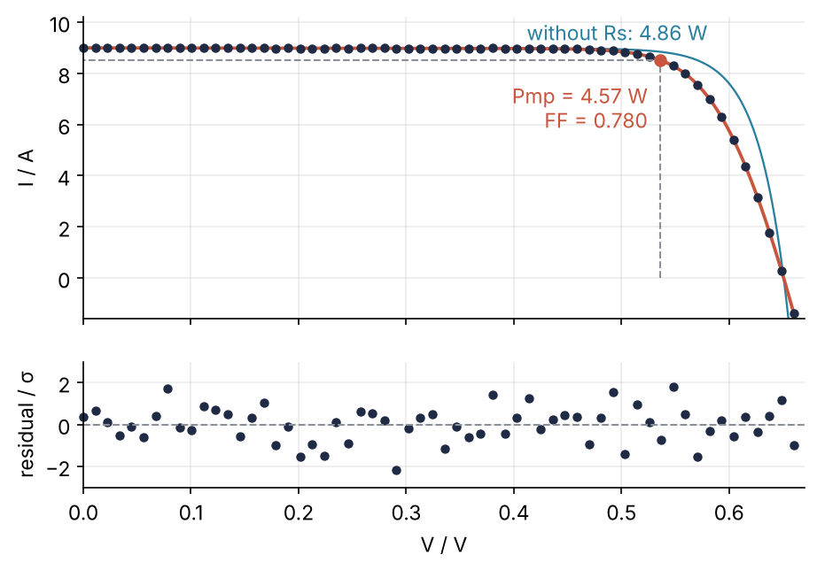
Current in A against voltage in V for a silicon cell. Dots: 60 measured points. Line: the single-diode fit. Thin line: the same cell without series resistance. The maximum power point is marked at 4.57 W, fill factor 0.780. Below: residuals in units of the 5 mA error, scattered without a pattern.

The fit runs through all 60 points, and the residuals scatter without a pattern. The cell delivers at most 4.57 W, with a fill factor of 0.780, the measure of how square the curve is: maximum power over short-circuit current times open-circuit voltage. Without its 4 mΩ of series resistance the same cell would give 0.29 W more.

Setup

The data come from the implicit equation itself, one root search per voltage with brentq between -2 and 10 A (Root finding with scipy.optimize), plus 5 mA of current noise from a seeded generator (Random numbers with numpy.random). The voltages carry no noise, which is what curve_fit assumes. The parameters list \(\ln I_0\) instead of \(I_0\), for a reason Step 3 gives. For your own cell, replace V and I with the measurement.

import numpy as np
import matplotlib.pyplot as plt
from scipy.optimize import curve_fit, brentq
from scipy.special import lambertw, wrightomega
from scipy.constants import k, e

plt.rcParams.update({
    "figure.figsize": (7, 3.6), "figure.dpi": 110,
    "axes.spines.top": False, "axes.spines.right": False,
    "axes.grid": True, "grid.alpha": 0.25,
    "font.size": 11, "lines.linewidth": 1.8,
})
INK, ACCENT, SECOND, MUTED = "#1f2a44", "#c8553d", "#2a7f9e", "#8a8f98"

T = 298.15                 # K, 25 °C
Vt = k * T / e             # thermal voltage, V
names = ["Iph", "lnI0", "n", "Rs", "Rsh"]
true = np.array([9.00, np.log(3e-10), 1.05, 4e-3, 20.0])   # A, ln(I0 / A), 1, ohm, ohm

def g(I, V, Iph, I0, n, Rs, Rsh, Vt=Vt):
    """Zero when I is the cell's current at the voltage V."""
    Vd = V + I * Rs                                        # across diode and shunt
    return Iph - I0 * np.expm1(Vd / (n * Vt)) - Vd / Rsh - I

def measure(V, Vt=Vt):
    Iph, lnI0, n, Rs, Rsh = true
    return np.array([brentq(g, -2, 10, args=(v, Iph, np.exp(lnI0), n, Rs, Rsh, Vt), xtol=1e-14)
                     for v in V])

rng = np.random.default_rng(7)
sigma = 5e-3                                               # A, the same for every point
V = np.linspace(0, 0.66, 60)
I_true = measure(V)
I = I_true + rng.normal(0, sigma, V.size)

print(f"{V.size} points, Isc = {I[0]:.2f} A, Voc = {np.interp(0, I[::-1], V[::-1]):.3f} V")

60 points, Isc = 9.00 A, Voc = 0.651 V

Step 1: Write the implicit equation and see why curve_fit cannot take it

curve_fit wants a model that takes the array of voltages and the parameters and returns the currents. The equation only gives \(g(I, V) = 0\). The honest workaround is a model that calls brentq once per voltage. Count what one call of it costs:

def current_by_root(V, Iph, lnI0, n, Rs, Rsh):
    currents, calls = [], 0
    for v in V:
        root, r = brentq(g, -2, 10, args=(v, Iph, np.exp(lnI0), n, Rs, Rsh), full_output=True)
        currents.append(root)
        calls += r.function_calls
    return np.array(currents), calls

_, calls = current_by_root(V, *true)
print(f"{calls} evaluations of g for one curve, {calls / V.size:.1f} per voltage")

332 evaluations of g for one curve, 5.5 per voltage

That alone is cheap. But unless it is handed a Jacobian, curve_fit finds the slopes of the model by finite differences: it calls the model again with each parameter nudged by a small step and divides the change in the currents by the step. Every iteration costs one model call per parameter on top of the first, six calls of 332 evaluations here, about 2,000. Worse, brentq finds each root only to its tolerance, so the root jitters from one nudge to the next, and the division by a small step turns that jitter into noise in the slopes. A model for a fit should be one vectorized expression in \(V\).

Step 2: Solve x = a + b exp(cx) with the Lambert W function

The Lambert W function is the inverse of \(w e^w\): \(W(z)\) is the \(w\) for which \(w e^w = z\). It solves one family of equations, those in which the unknown appears once outside an exponential and once, linearly, inside it:

\[x = a + b\,e^{cx} .\]

Substitute \(y = x - a\), which gives \(y = b\,e^{ca} e^{cy}\), and multiply both sides by \(-c\,e^{-cy}\). The left side becomes \(w e^w\) with \(w = -cy\), the right side the constant \(-bc\,e^{ca}\), so \(w = W(-bc\,e^{ca})\) and

\[x = a - \frac{W(-bc\,e^{ca})}{c} .\]

To bring your own equation there, collect every \(x\) outside the exponential on one side and every \(x\) inside it into one linear exponent. Whatever multiplies the exponential is \(b\).

The catch is the branches. For \(z \ge 0\), \(w e^w = z\) has one real solution, the principal branch \(k = 0\), which scipy.special.lambertw returns by default. Between \(-1/e\) and 0 a second one exists, the branch \(k = -1\), and below \(-1/e\) there is none. lambertw always returns a complex number, so take .real once you know your branch is real:

def w_solve(a, b, c):
    """The x that solves x = a + b*exp(c*x), on the principal branch of W."""
    return a - lambertw(-b * c * np.exp(c * a)).real / c

x = w_solve(2.0, -0.5, 0.3)
print(f"x = {x:.12f}   a + b exp(cx) = {2.0 - 0.5 * np.exp(0.3 * x):.12f}")

x = 1.268463480962   a + b exp(cx) = 1.268463480962

Both sides agree to the last digit printed.

Step 3: Write the cell's current in closed form

Now the cell. The shunt term holds an \(I\) outside the exponential, so collect it on the left and divide by \(1 + R_s/R_\mathrm{sh}\). The diode term splits into \(e^{V/(nV_t)}\), a constant for each point, times \(e^{IR_s/(nV_t)}\). That is the pattern of Step 2, with

\[a = \frac{R_\mathrm{sh}(I_\mathrm{ph} + I_0) - V}{R_s + R_\mathrm{sh}}, \qquad b = -\frac{I_0 R_\mathrm{sh}\,e^{V/(nV_t)}}{R_s + R_\mathrm{sh}}, \qquad c = \frac{R_s}{nV_t} ,\]

which is the explicit solution Jain and Kapoor published in 2004. Since \(b < 0\) and \(c > 0\), the argument of W is positive and the principal branch is the only real one. The model takes \(\ln I_0\) instead of \(I_0\): the saturation current is ten orders of magnitude below the photocurrent, and the fit nudges all parameters on comparable scales. Pitfall 1 shows what happens otherwise.

def cell_current(V, Iph, lnI0, n, Rs, Rsh):
    I0, nVt = np.exp(lnI0), n * Vt
    a = (Rsh * (Iph + I0) - V) / (Rs + Rsh)
    b = -I0 * Rsh * np.exp(V / nVt) / (Rs + Rsh)
    return w_solve(a, b, Rs / nVt)

print(f"largest difference from brentq: {np.max(np.abs(cell_current(V, *true) - I_true)):.1e} A")

largest difference from brentq: 9.3e-15 A

The closed form and the 60 root searches agree to 1e-14 A, a few roundings of a double near 9 A. The data were made by brentq, not by this formula, so the agreement checks the algebra.

Step 4: Read starting values off the slopes and fit

Five parameters with an exponential among them need a start near the answer. Each can be read off a part of the curve where one term dominates. Below 0.2 V the diode carries almost nothing, and the curve is the straight line \(I_\mathrm{ph} - V/R_\mathrm{sh}\): its intercept is \(I_\mathrm{ph}\), minus one over its slope is \(R_\mathrm{sh}\).

Near open circuit the slope \(-dV/dI\) is the series resistance plus the diode's own differential resistance. A diode whose current is \(I_0 e^{V/(nV_t)}\) has \(dI/dV\) equal to that current over \(nV_t\), so its resistance is \(nV_t\) divided by its current. At open circuit no current leaves the cell, the whole photocurrent flows through the diode, and the diode's resistance is \(nV_t/I_\mathrm{sc}\). Finally, open circuit means \(I_\mathrm{ph} \approx I_0 e^{V_\mathrm{oc}/(nV_t)}\), which gives \(\ln I_0\). Start \(n\) at 1.

low = V < 0.2
slope, Iph0 = np.polyfit(V[low], I[low], 1)
Voc0 = np.interp(0, I[::-1], V[::-1])
near = np.argsort(np.abs(V - Voc0))[:4]                  # the four points nearest open circuit
n0 = 1.0
Rs0 = -np.polyfit(I[near], V[near], 1)[0] - n0 * Vt / Iph0
p0 = [Iph0, np.log(Iph0) - Voc0 / (n0 * Vt), n0, Rs0, -1 / slope]

bounds = ([0, -60, 0.5, 0, 0], [np.inf, 0, 5, np.inf, np.inf])
popt, pcov = curve_fit(cell_current, V, I, p0=p0, sigma=np.full(V.size, sigma),
                       absolute_sigma=True, bounds=bounds)
chi2 = np.sum(((I - cell_current(V, *popt)) / sigma) ** 2)
dof = V.size - popt.size

units = ["A", "", "", "Ω", "Ω"]
for name, u, start, fit, t in zip(names, units, p0, popt, true):
    print(f"{name:4s} / {u:1s}  start {start:9.4g}   fit {fit:9.4g}   true {t:9.4g}")
print(f"chi2/dof = {chi2 / dof:.2f} for {dof} degrees of freedom")

Iph  / A  start     8.998   fit     8.998   true         9
lnI0 /    start    -23.13   fit    -21.98   true    -21.93
n    /    start         1   fit     1.048   true      1.05
Rs   / Ω  start  0.004558   fit  0.004006   true     0.004
Rsh  / Ω  start      18.6   fit        20   true        20
chi2/dof = 0.77 for 55 degrees of freedom

The start already lands close: 9.00 A, 18.6 Ω, and 4.6 mΩ against a fitted 4.0 mΩ, with \(\ln I_0\) off by 1.1 because \(n\) started at 1. Chi-square per degree of freedom is 0.77, about one standard deviation of \(\sqrt{2/55} = 0.19\) below 1: the error bars are right and the model fits, read as in curve_fit from the ground up.

Step 5: Read errors and the n-I0 correlation off the covariance

The standard errors are the square roots of the diagonal of pcov, the correlations its off-diagonal part scaled by them. Print both, and each parameter's miss from the truth, which only a simulation knows:

perr = np.sqrt(np.diag(pcov))
corr = pcov / np.outer(perr, perr)
for name, p, s, t in zip(names, popt, perr, true):
    print(f"{name:4s} = {p:10.5g} ± {s:.2g}   miss {(p - t) / s:+.2f} standard errors")
print(np.round(corr, 2))
print(f"r(n, ln I0) = {corr[1, 2]:.5f}   error ratio {perr[1] / perr[2]:.1f}"
      f"   Voc/(n² Vt) = {Voc0 / (popt[2] ** 2 * Vt):.1f}")

Iph  =     8.9982 ± 0.0017   miss -1.10 standard errors
lnI0 =     -21.98 ± 0.085   miss -0.62 standard errors
n    =     1.0477 ± 0.0037   miss -0.61 standard errors
Rs   =  0.0040062 ± 1.8e-05   miss +0.35 standard errors
Rsh  =     20.003 ± 2.2   miss +0.00 standard errors
[[ 1.   -0.34 -0.34  0.25 -0.89]
 [-0.34  1.    1.   -0.94  0.51]
 [-0.34  1.    1.   -0.94  0.51]
 [ 0.25 -0.94 -0.94  1.   -0.38]
 [-0.89  0.51  0.51 -0.38  1.  ]]
r(n, ln I0) = 0.99996   error ratio 23.1   Voc/(n² Vt) = 23.1

Every parameter lies within 1.1 standard errors of the truth, \(R_\mathrm{sh}\) to 11 %, \(R_s\) to 0.4 %. The correlation of \(n\) and \(\ln I_0\), 0.99996, is the physics and not a broken fit. Open circuit pins \(nV_t \ln(I_\mathrm{ph}/I_0)\), so a larger \(n\) drags \(\ln I_0\) along at \(d\ln I_0/dn = V_\mathrm{oc}/(n^2 V_t)\), which is 23.1, and the ratio of the two standard errors is 23.1 as well.

curve_fit from the ground up warns above 0.95. What decides whether a fit determined its parameters is the size of their errors, not \(r\). Its fit (c), four points below 2 mM, had \(K_m = 7.2 \pm 7.5\) mM with \(r = 0.998\), an error as large as the value. Here the curvature of the knee fixes \(n\) to 0.35 % and \(\ln I_0\) to 0.085, a 9 % error on \(I_0\). The correlation only says that \(I_0\) means nothing without its \(n\), so report both and \(r\). Refits to fresh noise check the errors:

refits = np.array([curve_fit(cell_current, V, I_true + rng.normal(0, sigma, V.size), p0=p0,
                             sigma=np.full(V.size, sigma), absolute_sigma=True, bounds=bounds)[0]
                   for _ in range(200)])
for name, s, spread in zip(names, perr, refits.std(axis=0, ddof=1)):
    print(f"{name:4s}  standard error {s:.3g}   spread of 200 refits {spread:.3g}")

Iph   standard error 0.00166   spread of 200 refits 0.00173
lnI0  standard error 0.0853   spread of 200 refits 0.0823
n     standard error 0.00369   spread of 200 refits 0.00358
Rs    standard error 1.78e-05   spread of 200 refits 1.65e-05
Rsh   standard error 2.15   spread of 200 refits 2.32

The spreads match the standard errors within 8 % for all five, which is as close as 200 refits can tell.

Step 6: Find the maximum power point and the series-resistance loss

The power is \(P = VI\). Evaluate the fitted curve on a grid of 10,001 voltages over the measured range, which runs past open circuit, and take the largest \(P\). The short-circuit current is the current at 0 V, the open-circuit voltage is where the current crosses zero, and the fill factor is \(FF = P_\mathrm{mp}/(I_\mathrm{sc} V_\mathrm{oc})\). Then the same cell without series resistance: the formula divides by \(R_s\), so pass 1e-12 Ω instead of zero.

Vg = np.linspace(0, 0.66, 10_001)
Ig = cell_current(Vg, *popt)
i = np.argmax(Vg * Ig)
Vmp, Imp, Pmp = Vg[i], Ig[i], Vg[i] * Ig[i]
Isc, Voc = Ig[0], np.interp(0, Ig[::-1], Vg[::-1])
FF = Pmp / (Isc * Voc)

I_ideal = cell_current(Vg, *popt[:3], 1e-12, popt[4])
P_ideal = np.max(Vg * I_ideal)
print(f"Vmp = {Vmp:.3f} V   Imp = {Imp:.2f} A   Pmp = {Pmp:.3f} W   FF = {FF:.3f}")
print(f"without Rs {P_ideal:.3f} W   loss {P_ideal - Pmp:.3f} W   Imp² Rs = {Imp ** 2 * popt[3]:.3f} W")

Vmp = 0.536 V   Imp = 8.51 A   Pmp = 4.567 W   FF = 0.780
without Rs 4.859 W   loss 0.292 W   Imp² Rs = 0.290 W

The maximum lies inside the grid at 0.536 V and 8.51 A. The series resistance costs 0.292 W, 6 % of the cell's power, and the Joule heat \(I_\mathrm{mp}^2 R_s\) of 0.290 W at the operating point says where it goes. The figure from the beginning:

fig, (ax, axr) = plt.subplots(2, 1, sharex=True, figsize=(7, 4.6),
                              gridspec_kw=dict(height_ratios=[2.4, 1]))
ax.plot(Vg, I_ideal, color=SECOND, lw=1.1)
ax.plot(Vg, Ig, color=ACCENT)
ax.plot(V, I, "o", color=INK, ms=4, clip_on=False)
ax.plot([Vmp, Vmp, 0], [0, Imp, Imp], ls="--", color=MUTED, lw=1)
ax.plot(Vmp, Imp, "o", color=ACCENT, ms=6, zorder=5)
ax.text(Vmp - 0.012, 7.6, f"Pmp = {Pmp:.2f} W\nFF = {FF:.3f}", ha="right", va="top", color=ACCENT)
ax.text(0.58, 9.3, f"without Rs: {P_ideal:.2f} W", ha="right", color=SECOND)
ax.set(ylabel="I / A", xlim=(0, 0.67), ylim=(-1.6, 10.2))

axr.plot(V, (I - cell_current(V, *popt)) / sigma, "o", color=INK, ms=4, clip_on=False)
axr.axhline(0, color=MUTED, ls="--", lw=1)
axr.set(xlabel="V / V", ylabel="residual / σ", ylim=(-3, 3))
fig.align_ylabels()
plt.show()

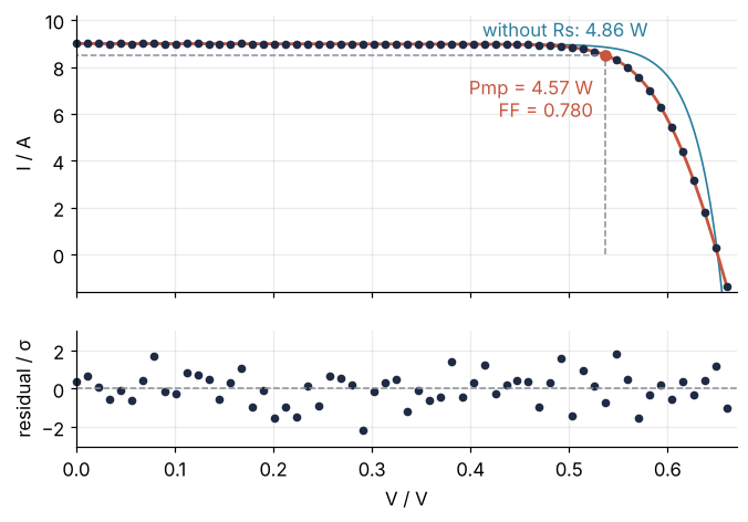
Current in A against voltage in V. Dots: 60 measured points. Line: the single-diode fit. Thin line: the cell without series resistance, 4.86 W. Dashed guides mark the maximum power point, 4.57 W, fill factor 0.780. Below: residuals in units of sigma, scattered between -2.2 and +1.8 without a pattern.

The two curves part only from the knee on, where the diode conducts and a shift of \(IR_s\), 36 mV at 9 A, moves the steep part of the curve sideways.

Pitfalls

Fitting \(I_0\) directly. Hand curve_fit the saturation current itself, started at the same place, and it stops early without complaint:

def cell_current_linear(V, Iph, I0, n, Rs, Rsh):
    return cell_current(V, Iph, np.log(I0), n, Rs, Rsh)

p0_lin = [p0[0], np.exp(p0[1]), *p0[2:]]
bounds_lin = ([0, 0, 0.5, 0, 0], [np.inf, np.inf, 5, np.inf, np.inf])
for diff_step in [None, 1e-8]:
    p, _ = curve_fit(cell_current_linear, V, I, p0=p0_lin, sigma=np.full(V.size, sigma),
                     absolute_sigma=True, bounds=bounds_lin, diff_step=diff_step)
    chi2_dof = np.sum(((I - cell_current_linear(V, *p)) / sigma) ** 2) / dof
    print(f"diff_step {str(diff_step):5s}  I0 = {p[1]:.3g} A   n = {p[2]:.3f}   chi2/dof = {chi2_dof:.2f}")
print(f"default nudge / I0 at the start: {np.sqrt(np.finfo(float).eps) / p0_lin[1]:.0f}")

diff_step None   I0 = 1e-10 A   n = 1.005   chi2/dof = 9.03
diff_step 1e-08  I0 = 2.85e-10 A   n = 1.048   chi2/dof = 0.77
default nudge / I0 at the start: 165

With the defaults it ends at \(I_0 = 1.0 \times 10^{-10}\) A and \(n = 1.005\) with chi-square per degree of freedom 9.0, no exception, no warning. The cause is the finite-difference nudge of Step 1: for a parameter below 1 it is about 1.5e-8 in absolute terms, 165 times the saturation current itself, so the slopes for \(I_0\) are measured across a step that changes the cell beyond recognition. diff_step=1e-8 makes the nudge relative and rescues this fit, which confirms the cause. Fit \(\ln I_0\), as in Step 3, and the problem never appears.

lambertw overflows for a module described as one cell. For the cell the argument of W stays below 7.1, with an exponent below 26. Feed the same formula a 60-cell module's voltages, 0 to 39.6 V, but keep the cell's \(nV_t\), as you do when you forget the number of cells, and the exponent reaches 1,468, far beyond the 709 at which np.exp returns inf:

V_module = 60 * V
with np.errstate(over="ignore", invalid="ignore"):
    print("lambertw:", cell_current(V_module[-3:], *true))
    try:
        curve_fit(cell_current, V_module, I, p0=true, bounds=bounds)
    except ValueError as err:
        print("curve_fit:", err)

def cell_current_omega(V, Iph, lnI0, n, Rs, Rsh):
    I0, nVt = np.exp(lnI0), n * Vt
    a = (Rsh * (Iph + I0) - V) / (Rs + Rsh)
    c = Rs / nVt
    ln_bc = lnI0 + np.log(Rsh * c / (Rs + Rsh)) + V / nVt     # ln(-bc) with the b of Step 3
    return a - wrightomega(ln_bc + c * a) / c                  # W(z) with ln z = ln(-bc) + ca

print("wrightomega:", np.round(cell_current_omega(V_module[-3:], *true), 1))
print(f"wrightomega on the cell, largest difference from brentq: "
      f"{np.max(np.abs(cell_current_omega(V, *true) - I_true)):.1e} A")

lambertw: [-inf -inf -inf]
curve_fit: Residuals are not finite in the initial point.
wrightomega: [-9354.8 -9522.5 -9690.2]
wrightomega on the cell, largest difference from brentq: 7.8e-15 A

The current comes out as minus infinity, and curve_fit refuses to start. The overflow sits in the argument \(z = -bc\,e^{ca}\) of Step 2, whose \(b\) carries \(e^{V/(nV_t)}\). wrightomega(x) equals \(W(e^x)\), so it takes \(x = \ln z = \ln(-bc) + ca\) instead, and with the \(b\) and \(c\) of Step 3, \(\ln(-bc) = \ln I_0 + \ln[R_\mathrm{sh} c/(R_s + R_\mathrm{sh})] + V/(nV_t)\) is a sum in which nothing is exponentiated. The currents are then finite at any voltage, if meaningless for a module described as one cell, and for the cell they agree with brentq as before.

For a module, the fix is the description, not the function. Give it \(N_s n V_t\) and the module's resistances, and ask how far a correctly described cell is from the overflow:

module = cell_current(V_module, *(true * [1, 1, 60, 60, 60]))   # n, Rs, Rsh for 60 cells in series
print(f"lambertw on the module as 60 cells, largest difference from the cell: {np.max(np.abs(module - I_true)):.1e} A")
Iph, lnI0, n, Rs, Rsh = true
Rpar = np.log(np.finfo(float).max) * n * Vt / Iph          # exp(ca) at 0 V overflows once Rs Rsh/(Rs + Rsh) passes this
print(f"lambertw overflows on this cell once Rs exceeds {Rpar * Rsh / (Rsh - Rpar):.2f} Ω")

lambertw on the module as 60 cells, largest difference from the cell: 1.3e-14 A
lambertw overflows on this cell once Rs exceeds 2.38 Ω

With the module described as 60 cells, \(a\), \(b\), and \(c\) are the cell's, and lambertw returns the cell's currents to 1.3e-14 A. A correctly described device overflows only when \(ca\) at 0 V, the voltage \(I_\mathrm{ph} R_s R_\mathrm{sh}/(R_s + R_\mathrm{sh})\) in units of \(nV_t\), passes 709, here at 2.38 Ω, about 600 times the true 4 mΩ. No working cell has that, so neither the cell nor the module needs wrightomega. The bounds leave \(R_s\) open above, though, and nothing stops a trial step of the fit from going there: when a fit from a poor start dies with non-finite residuals, use cell_current_omega as the model, which gives the same currents wherever lambertw gives any.

The thermal voltage at 25 °C for a hotter cell. Measure the same cell at 45 °C, keeping its \(I_0\) for simplicity although a real cell's rises steeply with temperature, and fit it with the \(V_t\) of 25 °C. The model only ever sees the product \(nV_t\), so the right temperature enters by scaling \(n\) by \(T_\mathrm{hot}/T\):

T_hot = 318.15
I_hot = measure(V, Vt=k * T_hot / e) + rng.normal(0, sigma, V.size)
fits = {"Vt at 25 °C": cell_current,
        "Vt at 45 °C": lambda V, Iph, lnI0, n, Rs, Rsh: cell_current(V, Iph, lnI0, n * T_hot / T, Rs, Rsh)}
for label, model in fits.items():
    p, c = curve_fit(model, V, I_hot, p0=p0, sigma=np.full(V.size, sigma), absolute_sigma=True, bounds=bounds)
    chi2_dof = np.sum(((I_hot - model(V, *p)) / sigma) ** 2) / dof
    print(f"{label}:  n = {p[2]:.3f} ± {np.sqrt(c[2, 2]):.3f}   chi2/dof = {chi2_dof:.2f}")
print(f"T_hot / T = {T_hot / T:.3f}")

Vt at 25 °C:  n = 1.121 ± 0.008   chi2/dof = 1.16
Vt at 45 °C:  n = 1.051 ± 0.007   chi2/dof = 1.16
T_hot / T = 1.067

With the wrong temperature \(n\) comes out 1.121 instead of 1.05, too large by the ratio of the two temperatures, 1.067, and chi-square is exactly as good as with the right one. The fit cannot notice. Measure the cell temperature and use it.

Variations

pvlib. pvlib.pvsystem.singlediode and pvlib.pvsystem.i_from_v solve the same equation, by default with Lambert W after Jain and Kapoor. i_from_v returns the current at given voltages, singlediode the short-circuit current, the open-circuit voltage, and the maximum power point. Use them to check your fit or to model a whole system.
A module. For \(N_s\) cells in series replace \(nV_t\) by \(N_s n V_t\) and read \(R_s\) and \(R_\mathrm{sh}\) as the module's. For identical cells the argument of W is then the cell's, and lambertw needs no help (Pitfall 2).
Temperature dependence. Fit curves measured at several cell temperatures, each with its own \(V_t\), and plot the fitted \(V_\mathrm{oc}\), \(I_0\), and \(P_\mathrm{mp}\) against temperature.
The two-diode model. A second diode with \(n = 2\) for recombination in the junction has no closed form with one W. Go back to the root search of Step 1, or give scipy.optimize.least_squares the implicit residual \(g\) with both \(I\) and the parameters as unknowns.

Cheat sheet

x = a - lambertw(-b * c * np.exp(c * a)).real / c         # solves x = a + b*exp(c*x), z >= 0: branch k = 0
a = (Rsh * (Iph + I0) - V) / (Rs + Rsh)                   # the single-diode cell
b = -I0 * Rsh * np.exp(V / (n * Vt)) / (Rs + Rsh)
c = Rs / (n * Vt)
lnz = np.log(I0 * Rsh * c / (Rs + Rsh)) + V / (n * Vt) + c * a   # log of the argument of W
I = a - wrightomega(lnz) / c                               # = a - W(z)/c, no overflow at any V
Rs0 = -dVdI_at_Voc - Vt / Isc                              # slope at Voc minus the diode's resistance, n0 = 1
popt, pcov = curve_fit(cell, V, I, p0=[intercept, lnI0_0, 1.0, Rs0, -1 / slope],   # line below 0.2 V
                       bounds=bounds, sigma=s, absolute_sigma=True)               # fit ln I0, never I0
P = Vg * cell(Vg, *popt); i = np.argmax(P); FF = P[i] / (Isc * Voc)