Profile likelihood: the lopsided error bar that curve_fit's ± hides (Python)

The question

A detector counts a short-lived isotope for 40 one-minute intervals. The first minute brings 61 counts, the last ones around 20, and about 15 of those per minute are background that would be there without the source. You want the half-life with an error bar. curve_fit gives a symmetric one, the profile likelihood a lopsided one, and 1000 simulated experiments at the end say which to trust.

Show code

import warnings

import numpy as np
import matplotlib.pyplot as plt
from scipy.optimize import curve_fit, least_squares, brentq
from scipy.special import xlogy

plt.rcParams.update({
    "figure.figsize": (7, 3.6), "figure.dpi": 110,
    "axes.spines.top": False, "axes.spines.right": False,
    "axes.grid": True, "grid.alpha": 0.25,
    "font.size": 11, "lines.linewidth": 1.8,
})
INK, ACCENT, SECOND, MUTED = "#1f2a44", "#c8553d", "#2a7f9e", "#8a8f98"

# Simulated from known values, so that every interval below can be checked against the truth.
A_true, T_true, B_true = 40.0, 10.0, 15.0        # counts/min, min, counts/min
rng = np.random.default_rng(320)
t = np.arange(40) + 0.5                           # middle of each one-minute interval / min


def rate(t, A, T, B):
    return A * 2.0 ** (-t / T) + B


N = rng.poisson(rate(t, A_true, T_true, B_true))


def deviance(N, mu):
    """The 40 terms of C, one per minute; xlogy makes a zero count contribute 0 ln 0 = 0."""
    return 2 * (mu - N + xlogy(N, N) - xlogy(N, mu))


def residuals(N, mu):
    """Signed square roots of the terms, so that least_squares, which sums squares, minimizes C."""
    return np.sign(N - mu) * np.sqrt(np.clip(deviance(N, mu), 0, None))


lower = [0, 0.1, 0]                               # no negative rate or background
fit = least_squares(lambda p: residuals(N, rate(t, *p)), x0=[40, 10, 15], bounds=(lower, np.inf))
best, C_min = fit.x, 2 * fit.cost
A_hat, T_hat, B_hat = best

# curve_fit at the same minimum, weighted with sigma = √μ as the Poisson counts demand
popt, pcov = curve_fit(rate, t, N, p0=best, sigma=np.sqrt(rate(t, *best)),
                       absolute_sigma=True, bounds=(lower, np.inf))
err = np.sqrt(np.diag(pcov))
corr = pcov / np.outer(err, err)
sigma_T = err[1]

t_fine = np.linspace(0, 40, 400)
fig, ax = plt.subplots()
ax.plot(t, N, "o", color=INK, ms=4)
ax.plot(t_fine, rate(t_fine, *best), color=ACCENT)
ax.axhline(B_true, color=MUTED, lw=1, ls="--")
ax.text(1, B_true - 1.5, "true background", color=MUTED, va="top")
ax.set(xlabel="t / min", ylabel="counts per minute", xlim=(0, 40), ylim=(0, 70))
plt.show()

for name, value, e, unit in zip(["A", "T½", "B"], popt, err, ["counts/min", "min", "counts/min"]):
    print(f"{name:2s} = {value:5.2f} ± {e:4.2f} {unit}")
print(f"correlation of T½ and B: {corr[1, 2]:+.2f}")

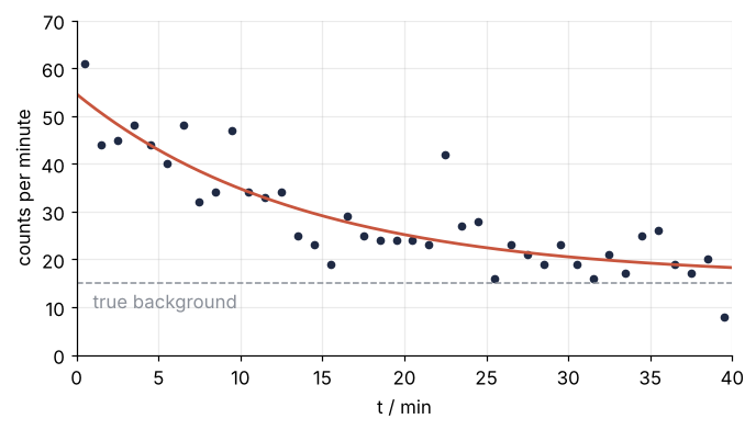
A  = 38.44 ± 3.70 counts/min
T½ =  9.56 ± 2.70 min
B  = 16.15 ± 3.09 counts/min
correlation of T½ and B: -0.92

The model is \(\mu(t) = A\,2^{-t/T_{1/2}} + B\): an initial rate \(A\), the half-life \(T_{1/2}\), and a background \(B\). The half-life is the parameter of interest. \(A\) and \(B\) are nuisance parameters: they must be fitted, but nobody wants them for themselves. The correlation of −0.92 between \(T_{1/2}\) and \(B\) says that a longer half-life can be traded for a lower background. The covariance behind those numbers is the one from curve_fit from the ground up.

The fit does not minimize \(\chi^2\) with \(\sqrt{N}\) error bars but its counting version. The likelihood is the probability of the 40 observed counts under the model: one Poisson probability per minute, all multiplied. The score \(C\) is \(-2\ln\) of that product, shifted so that a curve through every point would score 0. Lower is better, and for large counts \(C\) becomes the \(\chi^2\) you know.

A ± makes a promise you can test. For a \(\chi^2\) shaped like a perfect bowl, moving a parameter by one standard deviation and refitting the others costs exactly 1. So fix the half-life at either end of 9.56 ± 2.70 min, refit \(A\) and \(B\), and \(C\) should be worse than at the best fit by 1 on both sides:

Show code

def profile(T):
    """Fix the half-life at T, refit A and B; return the rise of C above its minimum and the refit (A, B)."""
    r = least_squares(lambda q: residuals(N, rate(t, q[0], T, q[1])), x0=[A_hat, B_hat], bounds=(0, np.inf))
    return 2 * r.cost - C_min, r.x


for side, T in [("short", T_hat - sigma_T), ("long", T_hat + sigma_T)]:
    print(f"{side:5s} end   T½ = {T:5.2f} min   C rises by {profile(T)[0]:.2f}   (the ± promises 1.00)")

short end   T½ =  6.86 min   C rises by 1.42   (the ± promises 1.00)
long  end   T½ = 12.26 min   C rises by 0.53   (the ± promises 1.00)

It is not: 1.42 on the short side, 0.53 on the long one. The data object to a short half-life more than the error bar says, and to a long one less. How far the half-life can move before \(C\) rises by 1, on each side separately, is the question the profile likelihood answers.

The idea: fix the half-life, let the rest refit

The procedure has four moves. Minimize \(C\) over all three parameters, which gives the best fit and the lowest score, \(C_\text{min}\). Fix the half-life at a trial value and minimize \(C\) over \(A\) and \(B\) alone. Record the rise above the minimum, \(\Delta C\): how much worse the data find that half-life when the other two parameters make the best of it. Repeat for every trial value. The curve of \(\Delta C\) against \(T_{1/2}\) is the profile likelihood, the profile for short, and the 68 % interval is where it stays below 1. A root finder searching on each side of the best fit finds the two crossings.

The second move is where the lopsidedness comes from. Each panel below fixes the half-life and plots \(\Delta C\) against the background, with \(A\) refit at every \(B\), so the lowest point of each curve is the profile at that half-life:

Show code

def slice_at(T, B):
    """Fix the half-life and the background, refit A alone: one point of a slice."""
    r = least_squares(lambda q: residuals(N, rate(t, q[0], T, B)), x0=[A_hat], bounds=(0, np.inf))
    return 2 * r.cost - C_min


B_grid = np.linspace(4, 28, 97)
fig, axes = plt.subplots(3, 1, figsize=(7, 6.4), sharex=True)
for ax, T in zip(axes, [7.0, T_hat, 14.0]):
    dC_T, (A_T, B_T) = profile(T)
    dC_T = max(dC_T, 0.0)                         # the refit at the best fit itself can land at -1e-9
    ax.plot(B_grid, [slice_at(T, B) for B in B_grid], color=ACCENT)
    ax.plot(B_T, dC_T, "o", color=ACCENT, ms=6)
    ax.axhline(1, color=MUTED, lw=1, ls="--")
    left = B_T > 14                               # the label goes on the side away from the minimum
    ax.text(0.02 if left else 0.98, 0.92, f"T½ = {T:.2f} min\nlowest ΔC = {dC_T:.2f}\nat B = {B_T:.1f}",
            transform=ax.transAxes, ha="left" if left else "right", va="top")
    ax.set(ylabel="ΔC", ylim=(0, 8))
axes[-1].set(xlabel="background B / counts per minute", xlim=(4, 28))
plt.show()

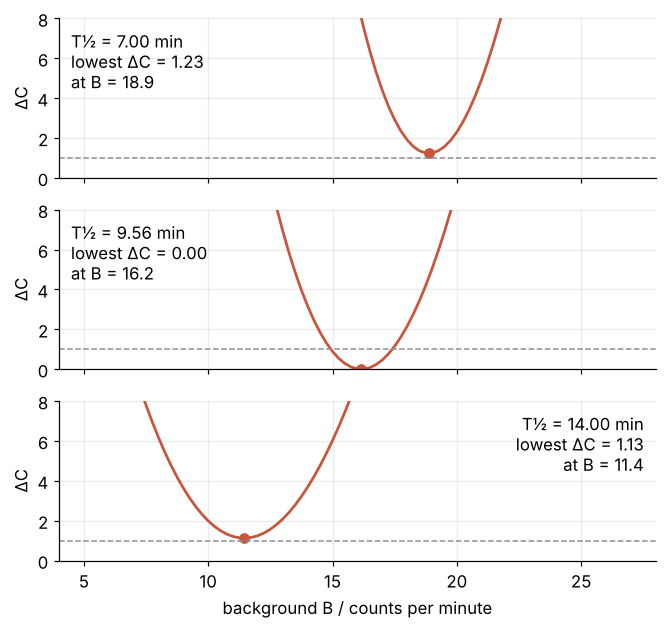
At 7.0 min the best background climbs to 18.9 counts per minute; at 14.0 min it drops to 11.4. A fast decay leaves the late counts to the background, and a slow one takes some of them over. The cost is not symmetric. Going 2.6 min shorter than the best fit costs \(\Delta C\) = 1.23, going 4.4 min longer only 1.13. The first minutes, at 61 and 44 counts, pin down how fast the decay can be, but a slow decay can hide in a lower background.

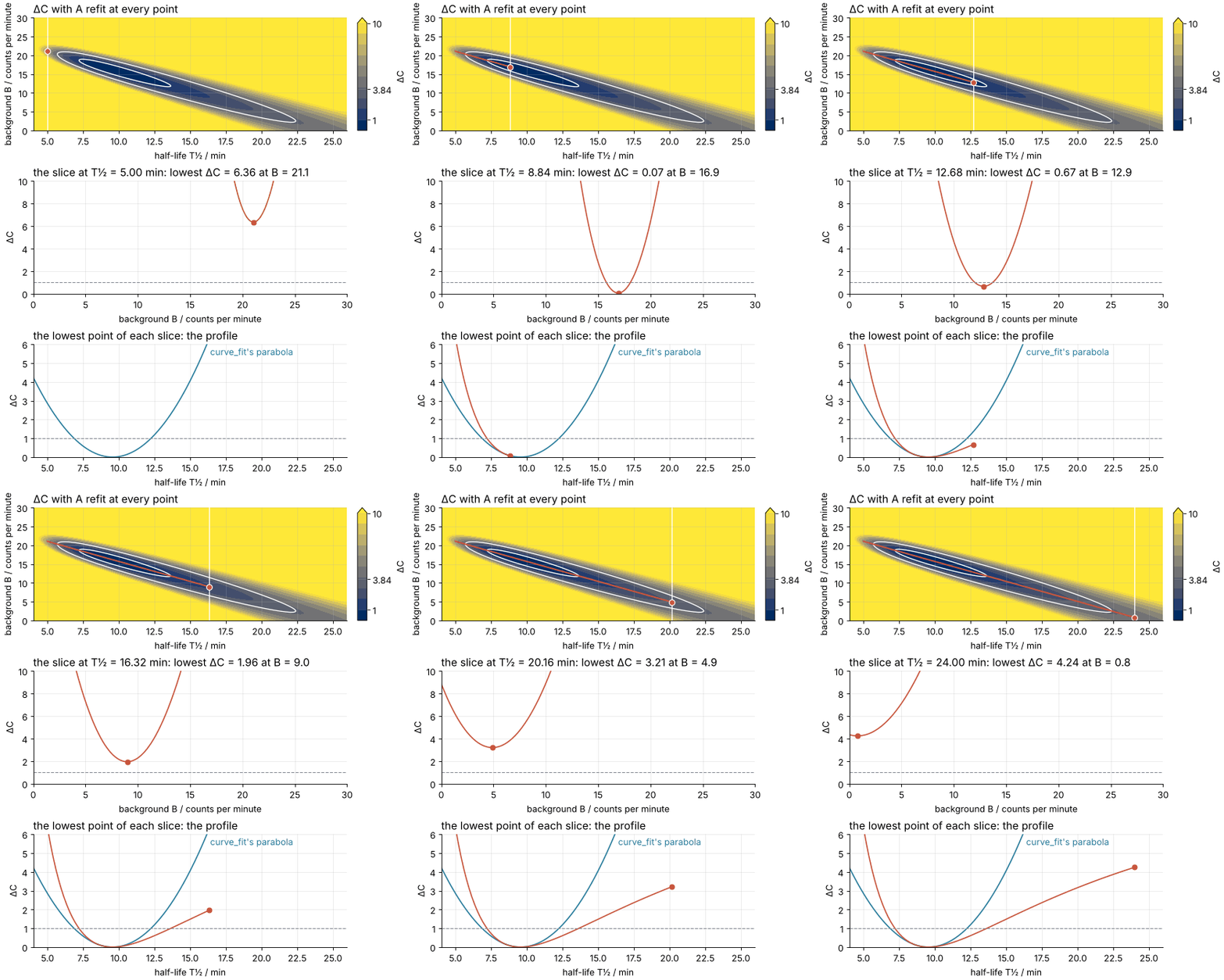
The animation sweeps the half-life from 5 to 24 min. Watch the bottom panel first, where the profile is traced out beside curve_fit's parabola. The middle panel is the current slice, \(\Delta C\) against \(B\). The top panel maps \(\Delta C\) over half-life and background, with \(A\) refit at every point and the cividis colormap dark where \(\Delta C\) is small; its dot, the slice minimum, slides down in \(B\) as the half-life grows.

Show code

"""Profile likelihood: fix the half-life, refit the rest, and trace the profile.

Renders ../../assets/profile-slice.gif. Run it from any directory:

    python scene.py
"""
from pathlib import Path

import numpy as np
import matplotlib.pyplot as plt
from matplotlib.animation import FuncAnimation, PillowWriter
from PIL import Image
from scipy.optimize import curve_fit, least_squares
from scipy.special import xlogy

OUT = Path(__file__).resolve().parents[2] / "assets" / "profile-slice.gif"
INK, ACCENT, SECOND, MUTED = "#1f2a44", "#c8553d", "#2a7f9e", "#8a8f98"
plt.rcParams.update({"axes.spines.top": False, "axes.spines.right": False,
                     "axes.grid": True, "grid.alpha": 0.25, "font.size": 11})

# ---- data: the counts of the tutorial, same seed, and the best fit
rng = np.random.default_rng(320)
t = np.arange(40) + 0.5                                              # min


def rate(t, A, T, B):
    return A * 2.0 ** (-t / T) + B


N = rng.poisson(rate(t, 40, 10, 15))


def C_of(mu):
    """The score C for every rate curve along the last axis."""
    return np.sum(2 * (mu - N + xlogy(N, N) - xlogy(N, mu)), axis=-1)


def residuals(p):
    mu = rate(t, *p)
    d = 2 * (mu - N + xlogy(N, N) - xlogy(N, mu))
    return np.sign(N - mu) * np.sqrt(np.clip(d, 0, None))


fit = least_squares(residuals, [40, 10, 15], bounds=([0, 0.1, 0], np.inf))
(A_hat, T_hat, B_hat), C_min = fit.x, 2 * fit.cost
_, pcov = curve_fit(rate, t, N, p0=fit.x, sigma=np.sqrt(rate(t, *fit.x)), absolute_sigma=True,
                    bounds=([0, 0.1, 0], np.inf))
sigma_T = np.sqrt(pcov[1, 1])                                        # curve_fit's σ of T½, for the parabola


def min_over_A(T, B, steps=30):
    """Fix T½ and B (arrays of equal shape), refit A by Newton's method on C; return ΔC."""
    g = 2.0 ** (-t / T[..., None])
    A = np.full(T.shape, A_hat)
    for _ in range(steps):
        mu = A[..., None] * g + B[..., None]
        A = np.clip(A - np.sum(g * (1 - N / mu), -1) / np.sum(N * g**2 / mu**2, -1), 1e-9, None)
    return C_of(A[..., None] * g + B[..., None]) - C_min


# ---- the map in the T½-B plane, and the slices along B
T_axis, B_axis = np.linspace(4, 26, 221), np.linspace(0, 30, 151)
TT, BB = np.meshgrid(T_axis, B_axis)
dC_map = min_over_A(TT, BB)
frames = np.linspace(5, 24, 100)                                     # the half-life, one value per frame
B_fine = np.linspace(0, 30, 1201)
slices = min_over_A(np.repeat(frames[:, None], B_fine.size, 1), np.tile(B_fine, (frames.size, 1)))
B_min, dC_prof = B_fine[slices.argmin(1)], slices.min(1)             # each slice's lowest point
T_fine = np.linspace(4, 26, 300)

# ---- figure, drawn once
# the colorbar gets a column of its own, so that the two half-life axes line up
fig, axd = plt.subplot_mosaic([["map", "bar"], ["slice", "."], ["prof", "."]], figsize=(7, 8.4), dpi=80,
                              width_ratios=[1, 0.03], layout="constrained")
ax1, ax2, ax3 = axd["map"], axd["slice"], axd["prof"]
cf = ax1.contourf(T_axis, B_axis, dC_map, levels=np.linspace(0, 10, 11), cmap="cividis", extend="max")
ax1.contour(T_axis, B_axis, dC_map, levels=[1, 3.84], colors="white", linewidths=1.2)
fig.colorbar(cf, cax=axd["bar"], label="ΔC", ticks=[1, 3.84, 10], format="%g")
vline = ax1.axvline(frames[0], color="white", lw=1.2)
(trail,) = ax1.plot([], [], color=ACCENT, lw=1.8)
(map_dot,) = ax1.plot([], [], "o", color=ACCENT, ms=7, mec="white")
ax1.set(xlabel="half-life T½ / min", ylabel="background B / counts per minute", xlim=(4, 26), ylim=(0, 30))
ax1.set_title("ΔC with A refit at every point", loc="left")

(slice_line,) = ax2.plot([], [], color=ACCENT)
(slice_dot,) = ax2.plot([], [], "o", color=ACCENT, ms=6)
ax2.axhline(1, color=MUTED, lw=1, ls="--")
ax2.set(xlabel="background B / counts per minute", ylabel="ΔC", xlim=(0, 30), ylim=(0, 10))
slice_title = ax2.set_title("", loc="left")                         # the numbers of the slice, set per frame

ax3.plot(T_fine, ((T_fine - T_hat) / sigma_T) ** 2, color=SECOND)
ax3.text(16.4, 5.6, "curve_fit's parabola", color=SECOND, va="center")
(prof_line,) = ax3.plot([], [], color=ACCENT)
(prof_dot,) = ax3.plot([], [], "o", color=ACCENT, ms=6)
ax3.axhline(1, color=MUTED, lw=1, ls="--")
ax3.set(xlabel="half-life T½ / min", ylabel="ΔC", xlim=(4, 26), ylim=(0, 6))
ax3.set_title("the lowest point of each slice: the profile", loc="left")


# ---- one frame: a function of the frame index alone
def update(i):
    T = frames[i]
    vline.set_xdata([T, T])
    trail.set_data(frames[: i + 1], B_min[: i + 1])
    map_dot.set_data([T], [B_min[i]])
    slice_line.set_data(B_fine, slices[i])
    slice_dot.set_data([B_min[i]], [dC_prof[i]])
    slice_title.set_text(f"the slice at T½ = {T:.2f} min: lowest ΔC = {dC_prof[i]:.2f} at B = {B_min[i]:.1f}")
    prof_line.set_data(frames[: i + 1], dC_prof[: i + 1])
    prof_dot.set_data([T], [dC_prof[i]])


# ---- render, and read back what was written
OUT.parent.mkdir(exist_ok=True)
FuncAnimation(fig, update, frames=frames.size).save(OUT, writer=PillowWriter(fps=12))
plt.close(fig)
with Image.open(OUT) as im:
    delay = im.info["duration"]
    print(f"{OUT.name}: {im.width} x {im.height} px, {im.n_frames} frames at {delay} ms, "
          f"{im.n_frames * delay / 1000:.1f} s, {OUT.stat().st_size / 1024:,.0f} kB")

Why curve_fit draws a parabola

curve_fit does not walk the valley. It measures how sharply \(C\) curves at the bottom in all three directions at once, a 3 × 3 matrix, halves it because \(C\) is twice the negative log-likelihood, and returns the inverse as pcov. Inverting the whole matrix is what lets \(A\) and \(B\) move along with the half-life. Near its minimum \(C\) is a quadratic bowl, and minimizing a quadratic bowl over two of its directions leaves a parabola in the third. Linear algebra says which one: \(\Delta C = ((T_{1/2} - \hat T_{1/2})/\sigma)^2\), with \(\sigma^2\) = pcov[1, 1], the matching diagonal entry of the inverse. So σ describes the profile at its bottom, with \(A\) and \(B\) refit. It is not the curvature of \(C\) along \(T_{1/2}\) with \(A\) and \(B\) held, which is about four times narrower and comes back in the Formalization.

curve_fit builds that matrix from the first derivatives of the model alone, the Gauss-Newton approximation: it drops the second derivatives and weights with the fitted rate instead of the counts, so it matches the exact curvature only approximately. Either way, what its ± describes is that parabola in place of the profile:

Show code

T_grid = np.linspace(4, 26, 200)
dC_profile = np.array([profile(T)[0] for T in T_grid])
dC_parabola = ((T_grid - T_hat) / sigma_T) ** 2


def ends(level):
    """Where the profile crosses the level, searched on each side of the best fit."""
    f = lambda T: profile(T)[0] - level
    return brentq(f, 3, T_hat), brentq(f, T_hat, 60)


prof_68, prof_95 = ends(1.0), ends(3.84)
para_68 = (T_hat - sigma_T, T_hat + sigma_T)
para_95 = (T_hat - 1.96 * sigma_T, T_hat + 1.96 * sigma_T)

h = 0.3                                           # curvature at the bottom, from three points of the profile
sigma_bottom = h * np.sqrt(2 / (profile(T_hat - h)[0] + profile(T_hat + h)[0]))

# the exact 3 × 3 curvature of C by central differences, inverted as a whole
C_at = lambda p: np.sum(deviance(N, rate(t, *p)))
step = 0.01 * np.eye(3)
H = np.array([[(C_at(best + si + sj) - C_at(best + si - sj) - C_at(best - si + sj) + C_at(best - si - sj))
               / (4 * 0.01**2) for sj in step] for si in step])
sigma_exact = np.sqrt(np.linalg.inv(H / 2)[1, 1])    # C is twice the negative log-likelihood

fig, ax = plt.subplots(figsize=(7, 3.8))
ax.plot(T_grid, dC_profile, color=ACCENT)
ax.plot(T_grid, dC_parabola, color=SECOND)
for level, share in [(1, "68 %"), (3.84, "95 %")]:
    ax.axhline(level, color=MUTED, lw=1, ls="--")
    ax.text(21, level + 0.08, share, color=MUTED, ha="right", va="bottom")
ax.axvline(T_true, color=MUTED, lw=1, ls="--")
ax.text(T_true + 0.2, 5.9, "true T½", color=MUTED, va="top")
for (lo, hi), color in [(prof_68, ACCENT), (para_68, SECOND)]:
    ax.plot([lo, hi], [1, 1], "o", color=color, ms=6)
ax.text(16.8, 5.9, f"curve_fit: {para_68[0]:.2f} to {para_68[1]:.2f} min", color=SECOND, va="top")
ax.text(16.8, 5.35, f"profile: {prof_68[0]:.2f} to {prof_68[1]:.2f} min", color=ACCENT, va="top")
ax.set(xlabel="half-life T½ / min", ylabel="ΔC", xlim=(4, 26), ylim=(0, 6))
plt.show()

print(f"σ from the profile's bottom: {sigma_bottom:.2f} min   from the inverted exact curvature: {sigma_exact:.2f} min"
      f"   curve_fit's: {sigma_T:.2f} min   (a step of {sigma_T:.2f} min on the {sigma_bottom:.2f} parabola: "
      f"ΔC = {(sigma_T / sigma_bottom) ** 2:.2f})")
print(f"68 %   profile {prof_68[0]:5.2f} to {prof_68[1]:5.2f} min   parabola {para_68[0]:5.2f} to {para_68[1]:5.2f} min"
      f"   profile as T½ = {T_hat:.2f} -{T_hat - prof_68[0]:.2f}/+{prof_68[1] - T_hat:.2f} min")
print(f"95 %   profile {prof_95[0]:5.2f} to {prof_95[1]:5.2f} min   parabola {para_95[0]:5.2f} to {para_95[1]:5.2f} min")
print(f"at T½ = 22 min   profile ΔC = {profile(22)[0]:.1f}   parabola ΔC = {((22 - T_hat) / sigma_T) ** 2:.1f}")

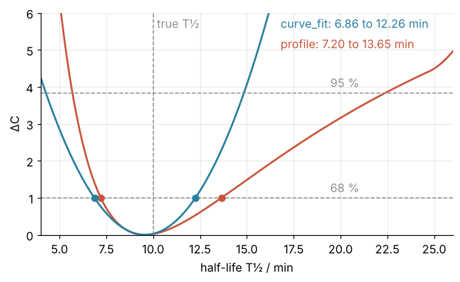
σ from the profile's bottom: 2.97 min   from the inverted exact curvature: 2.97 min   curve_fit's: 2.70 min   (a step of 2.70 min on the 2.97 parabola: ΔC = 0.83)
68 %   profile  7.20 to 13.65 min   parabola  6.86 to 12.26 min   profile as T½ = 9.56 -2.35/+4.09 min
95 %   profile  5.69 to 22.40 min   parabola  4.27 to 14.85 min
at T½ = 22 min   profile ΔC = 3.7   parabola ΔC = 21.2

Measured on the profile's own bottom, the curvature gives σ = 2.97 min, and inverting half the exact 3 × 3 curvature of \(C\) gives 2.97 min too, which is the linear algebra above at work. curve_fit's Gauss-Newton matrix gives 2.70 min: close, and just as symmetric. On the 2.97 parabola a step of 2.70 min costs 0.83, so part of the gap between 1.42 and 0.53 in the question is scale; the difference between the two sides is the lopsidedness. Away from the bottom the two curves part. At 22 min the parabola stands at 21.2, far outside any interval, and the profile at 3.7, inside the 95 % one. The 68 % interval moves from 6.86 to 12.26 min to 7.20 to 13.65 min, that is 9.56 −2.35/+4.09 min. At 95 % the profile reaches 22.40 min where the parabola stops at 14.85.

Formalization

The profile of the half-life is

\[\Delta C(T_{1/2}) = \min_{A,\,B}\; C(A, T_{1/2}, B) \;-\; C_\text{min}, \qquad C = 2\sum_i \left[\mu_i - N_i + N_i \ln\frac{N_i}{\mu_i}\right],\]

with \(N_i\) the counts and \(\mu_i\) the model's expected counts in minute \(i\). \(C\) is the Cash statistic, \(-2\ln\) of the Poisson likelihood up to a constant. Why not \(\chi^2\) with \(\sqrt{N}\) error bars? Because they give a low count a small error bar and so pull the fit down, the bias MCMC with emcee shows on the same kind of data. With Gaussian error bars the same recipe runs on \(\chi^2\) itself, with the same thresholds.

Wilks' theorem. Samuel Wilks showed in 1938 that at the true parameter value, with enough data, \(\Delta C\) behaves like the square of a standard normal miss, \(z^2\). That is the \(\chi^2\) distribution with one degree of freedom, one for the one parameter of interest. A miss within ±1σ means \(z^2 < 1\), which happens 68.3 % of the time; within ±1.96σ means \(z^2 < 3.84\), 95 % of the time. The thresholds 1 and 3.84 are those squares, and the theorem says the profile is the curve they apply to, not the parabola.

Coverage. The coverage of an interval method is the share of repeated experiments whose interval contains the true value. A 68 % method should catch the truth in 68 % of experiments, and you check that by simulation. Simulate many data sets from known parameters; on your own data, where the truth is unknown, simulate from your best fit, and again from the interval ends as other plausible truths. Rerun the whole analysis on each data set, fit and interval, and count the intervals that contain the value you simulated from. Split the misses into "truth below the interval" and "truth above it": a lopsided interval can reach the right total for the wrong reason, too long on one side and too short on the other. Then read the count against its own Monte Carlo error, \(\sqrt{p(1-p)/n}\), which is 1.5 percentage points for \(n\) = 1000 experiments at \(p\) = 68 % (Monte Carlo integration explains the square root).

Three consequences follow; the cell computes each on this data set.

Show code

fixed = lambda T: np.sum(deviance(N, rate(t, A_hat, T, B_hat))) - C_min
fix_68 = brentq(lambda T: fixed(T) - 1, 3, T_hat), brentq(lambda T: fixed(T) - 1, T_hat, 60)
print(f"A and B held at their best values: {fix_68[0]:.2f} to {fix_68[1]:.2f} min   "
      f"(width {fix_68[1] - fix_68[0]:.2f} min, profile {prof_68[1] - prof_68[0]:.2f} min)")


def rate_lambda(t, A, lam, B):                     # the same model in the decay constant λ = ln 2 / T½
    return A * np.exp(-lam * t) + B


p_lam, c_lam = curve_fit(rate_lambda, t, N, p0=[A_hat, np.log(2) / T_hat, B_hat],
                         sigma=np.sqrt(rate(t, *best)), absolute_sigma=True, bounds=(0, np.inf))
lam, s_lam = p_lam[1], np.sqrt(c_lam[1, 1])
print(f"profile in λ:   {np.log(2) / prof_68[1]:.4f} to {np.log(2) / prof_68[0]:.4f} per min"
      f"   back in T½: {prof_68[0]:.2f} to {prof_68[1]:.2f} min")
print(f"curve_fit in λ: {lam - s_lam:.4f} to {lam + s_lam:.4f} per min"
      f"   back in T½: {np.log(2) / (lam + s_lam):.2f} to {np.log(2) / (lam - s_lam):.2f} min")

# the wall: from which half-life on does the refit background sit at B = 0?
T_wall = brentq(lambda T: profile(T)[1][1] - 1e-3, T_hat, 26)
print(f"the refit background reaches B = 0 at T½ = {T_wall:.1f} min, where ΔC = {profile(T_wall)[0]:.2f}")

A and B held at their best values: 8.86 to 10.30 min   (width 1.44 min, profile 6.44 min)
profile in λ:   0.0508 to 0.0962 per min   back in T½: 7.20 to 13.65 min
curve_fit in λ: 0.0520 to 0.0930 per min   back in T½: 7.45 to 13.32 min
the refit background reaches B = 0 at T½ = 24.7 min, where ΔC = 4.42

Refit the nuisance parameters, never fix them. Holding \(A\) and \(B\) at their best values and moving only the half-life gives 8.86 to 10.30 min, an interval 1.44 min wide against the profile's 6.44 min. This is the curvature along \(T_{1/2}\) alone, and it ignores that the background can make room for a longer decay.

The interval does not depend on what you call the parameter. Fit the decay constant \(\lambda = \ln 2/T_{1/2}\) instead, and the profile interval is 0.0508 to 0.0962 per minute, which is exactly the same 7.20 to 13.65 min: fixing \(\lambda\) fixes \(T_{1/2}\), so the refits are identical. curve_fit's ± in \(\lambda\) maps back to 7.45 to 13.32 min, a third interval, neither the profile's nor its own 6.86 to 12.26 min. A parabola is a statement about one choice of axis.

Wilks needs many data and no walls. A wall is a bound a parameter sits on, here \(B = 0\). The theorem assumes that the best fit could move both ways, and at a wall it cannot. On these data the refit background reaches the wall at 24.7 min, which is the kink in the profile there, at \(\Delta C\) = 4.42, just past the 95 % threshold. Among the 1000 simulated experiments of the next section, 18 have their best background at 0. A separate run of curve_fit on those 18, without the bounds used everywhere else on this page, puts the background below 0 in all of them, down to −35.1 counts per minute. A wall away from the best fit can only make the profile rise faster on its side, because the refit loses room, so it pulls that interval end in, never out. Whether 1 and 3.84 then still cover is what a coverage check finds out, and the next section answers it for these data, wall experiments included.

See it in code

Show code

n_exp = 1000
N_sim = rng.poisson(rate(t, A_true, T_true, B_true), size=(n_exp, t.size))

# the best fit and curve_fit's σ, one experiment at a time, exactly as for the data above
best_sim, C_sim, cf_sim = np.empty((n_exp, 3)), np.empty(n_exp), np.empty((n_exp, 2))
for k, Nk in enumerate(N_sim):
    r = least_squares(lambda p: residuals(Nk, rate(t, *p)), x0=best, bounds=(lower, np.inf))
    best_sim[k], C_sim[k] = r.x, 2 * r.cost
    p, c = curve_fit(rate, t, Nk, p0=r.x, sigma=np.sqrt(rate(t, *r.x)), absolute_sigma=True,
                     bounds=(lower, np.inf))
    cf_sim[k] = p[1], np.sqrt(c[1, 1])


def profile_all(T, steps=25):
    """profile() for all experiments at once. At fixed T½ the rate is linear in A and B, so Newton's
    method on C converges in a few steps; a background pushed below 0 is set to 0, where the best A
    has a closed form."""
    g = 2.0 ** (-t / T[:, None])
    A, B = best_sim[:, 0], best_sim[:, 2]
    for _ in range(steps):
        mu = A[:, None] * g + B[:, None]
        grad_A, grad_B = np.sum((1 - N_sim / mu) * g, 1), np.sum(1 - N_sim / mu, 1)
        w = N_sim / mu**2
        H_AA, H_AB, H_BB = np.sum(w * g * g, 1), np.sum(w * g, 1), np.sum(w, 1)
        det = H_AA * H_BB - H_AB**2
        A, B = A - (H_BB * grad_A - H_AB * grad_B) / det, B - (H_AA * grad_B - H_AB * grad_A) / det
        wall = B < 0
        B = np.where(wall, 0.0, B)
        A = np.where(wall, N_sim.sum(1) / g.sum(1), A)
    return np.sum(deviance(N_sim, A[:, None] * g + B[:, None]), 1) - C_sim


def ends_all(level, far):
    """Bisection between each best fit and a far half-life, all experiments at once."""
    near, out = best_sim[:, 1].copy(), np.full(n_exp, far)
    for _ in range(40):
        mid = (near + out) / 2
        above = profile_all(mid) > level
        out, near = np.where(above, mid, out), np.where(above, near, mid)
    return (near + out) / 2


T_cf, s_cf = cf_sim.T
intervals = {
    "curve_fit T½ ± σ": (T_cf - s_cf, T_cf + s_cf),
    "profile, ΔC = 1": (ends_all(1.0, 0.5), ends_all(1.0, 200.0)),
    "curve_fit T½ ± 1.96σ": (T_cf - 1.96 * s_cf, T_cf + 1.96 * s_cf),
    "profile, ΔC = 3.84": (ends_all(3.84, 0.5), ends_all(3.84, 200.0)),
}
print(f"{'interval':22s} {'contains':>9s} {'truth below':>12s} {'truth above':>12s}")
for name, (lo, hi) in intervals.items():
    print(f"{name:22s} {100 * np.mean((lo <= T_true) & (T_true <= hi)):7.1f} % "
          f"{100 * np.mean(T_true < lo):10.1f} % {100 * np.mean(hi < T_true):10.1f} %")
for p in [0.683, 0.95]:
    print(f"Monte Carlo error at {100 * p:.1f} %: {100 * np.sqrt(p * (1 - p) / n_exp):.1f} points")
print(f"curve_fit ± 1.96σ intervals with a negative lower end: {np.sum(T_cf - 1.96 * s_cf < 0)}")

# a separate run: the experiments whose best background sits on the wall, refit without bounds
at_wall = best_sim[:, 2] < 1e-6
with warnings.catch_warnings():
    warnings.simplefilter("ignore")               # 2**(-t/T) overflows on the way for some starts
    B_free = np.array([curve_fit(rate, t, Nk, p0=[40, 10, 15], sigma=np.sqrt(rate(t, *b)),
                                 absolute_sigma=True)[0][2] for Nk, b in zip(N_sim[at_wall], best_sim[at_wall])])
print(f"best background at the wall B = 0: {at_wall.sum()} of {n_exp}; "
      f"without bounds curve_fit puts it below 0 in {np.sum(B_free < 0)}, down to {B_free.min():.1f} counts/min")

fig, axes = plt.subplots(2, 1, figsize=(7, 5.6), sharex=True)
for ax, name, color in zip(axes, ["curve_fit T½ ± σ", "profile, ΔC = 1"], [SECOND, ACCENT]):
    lo, hi = intervals[name]
    for k in range(30):
        miss = not lo[k] <= T_true <= hi[k]
        ax.plot([lo[k], hi[k]], [k, k], color=color, lw=1.6, alpha=1 if miss else 0.35)   # misses in full color
    ax.vlines(T_true, -1, 30, color=MUTED, lw=1, ls="--")
    ax.text(0.01, 0.98, f"{name}: contains {100 * np.mean((lo <= T_true) & (T_true <= hi)):.1f} % of {n_exp}\n"
            f"misses (full color): truth below {100 * np.mean(T_true < lo):.1f} %, above {100 * np.mean(hi < T_true):.1f} %",
            transform=ax.transAxes, va="top")
    ax.set(ylabel="experiment", ylim=(-1, 42), yticks=[0, 10, 20, 30])
axes[-1].set(xlabel="half-life T½ / min", xlim=(0, 30))
plt.show()

interval                contains  truth below  truth above
curve_fit T½ ± σ          76.8 %        3.5 %       19.7 %
profile, ΔC = 1           67.9 %       17.0 %       15.1 %
curve_fit T½ ± 1.96σ      91.7 %        0.0 %        8.3 %
profile, ΔC = 3.84        94.5 %        2.4 %        3.1 %
Monte Carlo error at 68.3 %: 1.5 points
Monte Carlo error at 95.0 %: 0.7 points
curve_fit ± 1.96σ intervals with a negative lower end: 34
best background at the wall B = 0: 18 of 1000; without bounds curve_fit puts it below 0 in 18, down to -35.1 counts/min

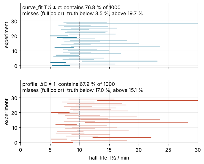
The profile catches the truth in 67.9 % of the 1000 experiments at the 68 % level and in 94.5 % at the 95 % level, both within their Monte Carlo errors of 1.5 and 0.7 points. Its misses split about evenly, 17.0 % with the truth below and 15.1 % above, where 15.9 % each is expected.

curve_fit's ± σ contains the truth in 76.8 %, more than promised, but for the wrong reason: the truth lies below it in only 3.5 % of experiments and above it in 19.7 %. Its interval is too long on the short side and too short on the long one, which is the asymmetry of the single data set, repeated a thousand times. At ± 1.96σ the error shows in the total as well: 91.7 % instead of 95 %, with every miss on the long side, while 34 of the intervals start at a negative half-life.

Where it shows up

Every field that fits a model with parameters it does not care about meets the same choice between the curvature at the minimum and the profile.

Particle physics. MINUIT, the minimizer CERN has distributed since the 1970s, has two error commands: HESSE inverts the curvature matrix as curve_fit does, and MINOS walks the profile on each side and reports asymmetric errors. The Higgs discovery in 2012 was claimed with test statistics built from the profile likelihood ratio, with the detector systematics as nuisance parameters.
X-ray and gamma-ray astronomy. Cash introduced the statistic used here, up to a constant, in 1979 for photon counts with few events per bin. XSPEC, the standard X-ray spectral fitting program, computes parameter errors by stepping one parameter and refitting the rest until the statistic rises by 2.706, the 90 % threshold.
Systems biology. Models of signaling pathways have dozens of rate constants and few measured species. Raue and coworkers made the profile a standard test of practical identifiability: a parameter whose profile never crosses the threshold on one side is not determined by the data at all, something a covariance matrix cannot say.
Pharmacokinetics. Clearance and volume of distribution are fitted from a few blood samples per patient, and their intervals are often asymmetric. PsN, the toolkit around the population modeling program NONMEM, offers log-likelihood profiling as the alternative to the standard errors of NONMEM's covariance step.
Enzyme kinetics. \(K_m\) and \(V_\text{max}\) of Michaelis-Menten kinetics trade against each other when the substrate concentrations do not reach well past \(K_m\), the same situation as half-life and background here (curve_fit from the ground up fits that model).
Cosmology. The Planck collaboration published profile likelihoods of cosmological parameters next to its Bayesian posteriors, to check that the priors did not drive the result.

In each case the rule is the one this data set showed. A straight trade between parameters, a tilted bowl, is what pcov handles. It cannot handle a \(C\) that is no bowl in the parameter of interest even with the trade followed. Here a short half-life must explain the 61 and 44 counts of the first minutes, while a long one can pass counts to the background, so the profile is steep on one side and shallow on the other: 1.23 at 2.6 min shorter, 1.13 at 4.4 min longer. Few counts make that worse. A wall is a separate case that adds a kink of its own, here at 24.7 min, outside the 68 % interval. Compute the profile, and if it crosses 1 at different distances on the two sides, report the profile.

The question

The idea: fix the half-life, let the rest refit

Why curve_fit draws a parabola

Formalization

See it in code

Where it shows up

Further reading