Clebsch-Gordan coefficients with sympy.physics.wigner: the sodium D lines

The problem: why is sodium's D2 line twice as strong as D1?

A sodium lamp glows in two yellow lines, D2 at 589.0 nm and D1 at 589.6 nm (wavelengths in air), and D2 is twice as strong as D1. Both facts come from one electron in a 3p orbital whose orbital angular momentum \(l = 1\) couples with its spin \(1/2\), and the numbers that describe that coupling are the Clebsch-Gordan coefficients. They are square roots of rationals. Books tabulate them, readers copy them with sign errors, and a computer in floating point turns a selection rule into 1e-17 instead of zero.

In term symbols the lower level is 3s ²S₁/₂ and the two upper levels are 3p ²P₁/₂ and ²P₃/₂. The superscript is \(2S+1\), the letter S, P, D stands for \(L = 0, 1, 2\), and the subscript is \(J\), so ²P₃/₂ has \(S = 1/2\), \(L = 1\), and \(J = 3/2\). Capitals are the angular momenta of the whole atom; sodium's closed shells add nothing, so here they equal the valence electron's \(l\), \(s\), and \(j\). D1 is ²P₁/₂ → ²S₁/₂ and D2 is ²P₃/₂ → ²S₁/₂. sympy.physics.wigner computes every coefficient exactly. With three of its functions, clebsch_gordan, wigner_3j, and wigner_6j, you get the coupled states of the 3p electron, the 2 : 1 ratio from a 6j symbol, the Landé factors, and the splitting of each line in a weak magnetic field into four and six components. The same three calls work for any transition between two levels labeled this way.

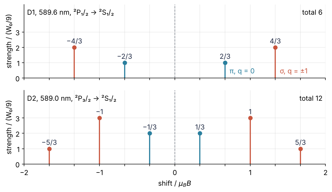
Zeeman components of the sodium D lines in a weak field, strength against shift in units of μ_B B. D1: four components, π at ±2/3, σ at ±4/3. D2: six, π at ±1/3, σ at ±1 and ±5/3. The D2 strengths add up to twice those of D1.

Each stem is one transition from an upper sublevel \(M'\) to a lower sublevel \(M\): its position comes from the Landé factors, its height from a 3j symbol, and Step 5 draws it. The SymPy you need is in SymPy from the ground up.

Setup

h is the only half-integer typed by hand; every other one is built from it or from Rational, so everything below stays exact.

import sympy as sp
from sympy import S, Rational, sqrt
from sympy.physics.wigner import clebsch_gordan, wigner_3j, wigner_6j
from sympy.physics.quantum.cg import CG
import scipy.constants as const
import matplotlib.pyplot as plt

h = S.Half                    # an exact 1/2; never 0.5 or 1/2 (see Pitfalls)

def mvals(J):
    """The magnetic quantum numbers J, J - 1, ..., -J."""
    return [J - k for k in range(int(2 * J) + 1)]

plt.rcParams.update({
    "figure.figsize": (7.5, 4.4), "figure.dpi": 110,
    "axes.spines.top": False, "axes.spines.right": False,
    "axes.grid": True, "grid.alpha": 0.25,
    "font.size": 11, "lines.linewidth": 1.8,
})
INK, ACCENT, SECOND, MUTED = "#1f2a44", "#c8553d", "#2a7f9e", "#8a8f98"

print("SymPy", sp.__version__, "  <1 0; 1/2 1/2 | 3/2 1/2> =", clebsch_gordan(1, h, Rational(3, 2), 0, h, h))

SymPy 1.14.0   <1 0; 1/2 1/2 | 3/2 1/2> = sqrt(6)/3

Step 1: Couple l = 1 and s = 1/2 with clebsch_gordan

The arguments of clebsch_gordan(j1, j2, J, m1, m2, M) are the two angular momenta, the total, and then the three projections. The value is \(\langle l\, m_l; s\, m_s | J\, M\rangle\), the amplitude of the uncoupled state \(|m_l, m_s\rangle\) in the coupled state \(|J, M\rangle\). The setup printed one of them. The class CG from sympy.physics.quantum.cg holds the same number with the arguments in pairs, \((j_1, m_1, j_2, m_2, J, M)\), and stays unevaluated inside quantum expressions until you call .doit():

c = CG(1, 0, h, h, Rational(3, 2), h)
print(c, "=", c.doit())

CG(1, 0, 1/2, 1/2, 3/2, 1/2) = sqrt(6)/3

Now all six coupled states. The loop prints each as a sum of uncoupled kets and fills the matrix U, one row per coupled state, one column per uncoupled state:

uncoupled = [(ml, ms) for ml in (1, 0, -1) for ms in (h, -h)]      # columns of U
coupled = [(J, M) for J in (Rational(3, 2), h) for M in mvals(J)]   # rows of U
arrow = {h: "↑", -h: "↓"}

U = sp.zeros(6, 6)
for i, (J, M) in enumerate(coupled):
    terms = []
    for k, (ml, ms) in enumerate(uncoupled):
        U[i, k] = clebsch_gordan(1, h, J, ml, ms, M)
        if U[i, k] != 0:
            terms.append(f"({U[i, k]}) |{ml},{arrow[ms]}⟩")
    print(f"|{J}, {str(M):>4s}⟩ = " + " + ".join(terms))

|3/2,  3/2⟩ = (1) |1,↑⟩
|3/2,  1/2⟩ = (sqrt(3)/3) |1,↓⟩ + (sqrt(6)/3) |0,↑⟩
|3/2, -1/2⟩ = (sqrt(6)/3) |0,↓⟩ + (sqrt(3)/3) |-1,↑⟩
|3/2, -3/2⟩ = (1) |-1,↓⟩
|1/2,  1/2⟩ = (sqrt(6)/3) |1,↓⟩ + (-sqrt(3)/3) |0,↑⟩
|1/2, -1/2⟩ = (sqrt(3)/3) |0,↓⟩ + (-sqrt(6)/3) |-1,↑⟩

So \(|3/2, 1/2\rangle = \sqrt{1/3}\,|1,\downarrow\rangle + \sqrt{2/3}\,|0,\uparrow\rangle\). The stretched states \(|3/2, \pm 3/2\rangle\) have a single term, and the \(J = 1/2\) states carry a minus sign, which is the Condon-Shortley phase convention SymPy follows. Printed as a matrix, U should be a proper change of basis:

sp.pprint(U)
print("U U^T == 1:", U * U.T == sp.eye(6))

⎡1  0    0    0    0    0⎤
⎢                        ⎥
⎢   √3   √6              ⎥
⎢0  ──   ──   0    0    0⎥
⎢   3    3               ⎥
⎢                        ⎥
⎢             √6   √3    ⎥
⎢0  0    0    ──   ──   0⎥
⎢             3    3     ⎥
⎢                        ⎥
⎢0  0    0    0    0    1⎥
⎢                        ⎥
⎢   √6  -√3              ⎥
⎢0  ──  ────  0    0    0⎥
⎢   3    3               ⎥
⎢                        ⎥
⎢             √3  -√6    ⎥
⎢0  0    0    ──  ────  0⎥
⎣             3    3     ⎦
U U^T == 1: True

True, exactly, where floats would need a tolerance. The coupled states are a new orthonormal basis of the same six states, and the zeros show that only kets with equal \(M = m_l + m_s\) mix. Step 4 reuses U.

Step 2: Write transition amplitudes as 3j symbols

A photon carries angular momentum 1, so emitting one couples three angular momenta: the upper level's \(J'\), the photon's 1, and the lower level's \(J\). Physics books write that coupling as a Wigner 3j symbol, which is a Clebsch-Gordan coefficient rearranged to be symmetric in all three. The heights in the figure above are its squares.

The Wigner-Eckart theorem says where the dependence on the sublevels sits. In Edmonds' convention, for a component \(q\) of the dipole operator \(d\),

\[\langle J' M' | d_q | J M\rangle = (-1)^{J'-M'} \begin{pmatrix} J' & 1 & J \\ -M' & q & M \end{pmatrix} \langle J' \| d \| J\rangle .\]

Everything about \(M'\), \(M\), and \(q\) is in the 3j symbol. Everything about the atom, the radial wave functions and the charge, is in the reduced matrix element \(\langle J' \| d \| J\rangle\), one number per pair of levels. The 3j symbol vanishes unless \(q = M' - M\), the photon's angular momentum along the field: the \(\Delta m = 0, \pm 1\) rule you know from hydrogen. The conversion to Clebsch-Gordan coefficients is

\[\langle j_1 m_1; j_2 m_2 | J M\rangle = (-1)^{j_1 - j_2 + M} \sqrt{2J+1} \begin{pmatrix} j_1 & j_2 & J \\ m_1 & m_2 & -M \end{pmatrix} .\]

Check it on all 36 entries of U, then ask for two forbidden transitions. The last loop tests the claim that the 3j squares only share a line's strength out among its components. If they favor no upper sublevel, the components leaving each \(M'\) add up to the same total:

def cg_from_3j(j1, j2, J, m1, m2, M):
    return (-1)**(j1 - j2 + M) * sqrt(2 * J + 1) * wigner_3j(j1, j2, J, m1, m2, -M)

mismatches = sum(cg_from_3j(1, h, J, ml, ms, M) != U[i, k]
                 for i, (J, M) in enumerate(coupled) for k, (ml, ms) in enumerate(uncoupled))
print("mismatches with U:", mismatches)
print("M' - M = 2: ", wigner_3j(Rational(3, 2), 1, h, -Rational(3, 2), 2, -h))
print("J' - J = 2: ", wigner_3j(Rational(5, 2), 1, h, -h, 0, h))

for Ju in (h, Rational(3, 2)):
    sums = [sum(wigner_3j(Ju, 1, h, -Mu, q, Mu - q)**2 for q in (-1, 0, 1)) for Mu in mvals(Ju)]
    print(f"J' = {Ju}: sum over components, one per M' =", sums)

mismatches with U: 0
M' - M = 2:  0
J' - J = 2:  0
J' = 1/2: sum over components, one per M' = [1/2, 1/2]
J' = 3/2: sum over components, one per M' = [1/4, 1/4, 1/4, 1/4]

The selection rules are exact zeros. The sums are \(1/2\) for both sublevels of ²P₁/₂ and \(1/4\) for all four of ²P₃/₂, which is \(1/(2J'+1)\) and the same for every \(M'\). A decay rate goes as the squared dipole matrix element, so every sublevel of a level decays equally fast, and all components together add up to \(|\langle J' \| d \| J\rangle|^2\), the strength of the whole line.

Step 3: Get the 2 : 1 ratio from a 6j symbol

The reduced element of Step 2 connects levels \(|(L S) J\rangle\), but the dipole operator acts on the orbital motion only, and the spin \(S\) is a spectator. The transition is simple when the photon's 1 couples to \(L\) first, giving \(L'\), and the spin joins afterwards to give \(J'\). The levels are built in the other order: \(L\) with \(S\) to \(J\), then the photon to \(J'\). Step 1's U held the overlaps between two bases of the same states, \(l\) and \(s\) apart or coupled. A 6j symbol is the same kind of overlap between these two orders of coupling \(L\), \(S\), and 1, up to a sign and a factor \(\sqrt{(2L'+1)(2J+1)}\). Squared, it shares \(2S+1\) times the orbital strength among the pairs of \(J\) levels.

Its six slots hold the six angular momenta as \(\{L'\ J'\ S;\ J\ L\ 1\}\), arranged so that each of its four triangles is one coupling: \((J\,L\,S)\) the lower level, \((L'\,L\,1)\) the orbital transition, \((L'\,J'\,S)\) the upper level, and \((J\,J'\,1)\) the transition between the \(J\) levels. That is how you fill it for any transition. With \(W\) for a line strength, to keep \(S\) for the spin,

\[W(J \to J') = (2J+1)(2J'+1) \begin{Bmatrix} L' & J' & S \\ J & L & 1 \end{Bmatrix}^2 W_0, \qquad W_0 = |\langle L' \| d \| L\rangle|^2 .\]

For sodium, \(L = 0\), \(L' = 1\), and \(S = J = 1/2\):

def line_strength(Lu, Ju, Ll, Jl, spin):
    """Strength of (Lu spin) Ju -> (Ll spin) Jl, in units of W0 = |<Lu||d||Ll>|^2."""
    return (2 * Jl + 1) * (2 * Ju + 1) * wigner_6j(Lu, Ju, spin, Jl, Ll, 1)**2

for name, Ju in [("D1", h), ("D2", Rational(3, 2))]:
    six = wigner_6j(1, Ju, h, h, 0, 1)
    print(f"{name}: 6j = {str(six):>10s}   W = {line_strength(1, Ju, 0, h, h)} W0")
print("D2 / D1 =", line_strength(1, Rational(3, 2), 0, h, h) / line_strength(1, h, 0, h, h))

D1: 6j =  sqrt(6)/6   W = 2/3 W0
D2: 6j = -sqrt(6)/6   W = 4/3 W0
D2 / D1 = 2

The two 6j symbols differ only in sign, so the ratio is \((2 \cdot 3/2 + 1)/(2 \cdot 1/2 + 1) = 2\), the count of upper sublevels. An absorption oscillator strength is proportional to \(W\) times the transition frequency over the lower level's \(2J+1\). Both lines share that level and differ in frequency by 0.1 %, so Steck's values for sodium, 0.6405 and 0.3199, keep the ratio at 2.002. Books normalize reduced matrix elements differently, by factors of \(2J+1\) and a sign, but never the ratio.

Step 4: Derive the Landé factors from the coupled states

In a weak field the Zeeman energy is first-order perturbation theory: the expectation value of \(\mu_B B (L_z + g_s S_z)\) in the unperturbed state \(|J, M\rangle\), with \(g_s = 2\). It comes out as \(g_J \mu_B B M\). Step 1's expansions give it directly, as \(\sum c^2 (m_l + 2 m_s)/M\) over the entries \(c\) of the row of U for \(M = 1/2\), and the textbook formula gives it in one line:

for J in (Rational(3, 2), h):
    i = coupled.index((J, h))
    g = sum(U[i, k]**2 * (ml + 2 * ms) for k, (ml, ms) in enumerate(uncoupled)) / h
    print(f"from the expansion of |{J}, 1/2>: g_J = {g}")

def g_J(L, spin, J, g_s=2):
    return 1 + (g_s - 1) * (J * (J + 1) + spin * (spin + 1) - L * (L + 1)) / (2 * J * (J + 1))

print("formula, 2P3/2  2P1/2  2S1/2:", g_J(1, h, Rational(3, 2)), g_J(1, h, h), g_J(0, h, h))
g_e = abs(const.physical_constants["electron g factor"][0])
print(f"with g_s = {g_e:.5f}:        {g_J(1, h, Rational(3, 2), g_e):.4f} {g_J(1, h, h, g_e):.4f}")

from the expansion of |3/2, 1/2>: g_J = 4/3
from the expansion of |1/2, 1/2>: g_J = 2/3
formula, 2P3/2  2P1/2  2S1/2: 4/3 2/3 2
with g_s = 2.00232:        1.3341 0.6659

The two routes agree exactly: \(4/3\), \(2/3\), and 2 for the ground state. With the measured electron \(g\) factor from scipy.constants the P levels move in the fourth digit, which the figure does not resolve.

Step 5: Draw the Zeeman pattern with 3j weights

Steps 2 to 4 combine into one recipe for an upper level \((L' S) J'\) and a lower level \((L S) J\) with the same spin:

the line strength is line_strength(L′, J′, L, J, S) from Step 3;
a component \(M' \to M\) exists for \(q = M' - M \in \{-1, 0, 1\}\) and has the strength \(W \cdot (J'\ 1\ J;\ -M'\ q\ M)^2\) from Step 2;
it is shifted by \((g_{J'} M' - g_J M)\, \mu_B B\) from Step 4;
it is a π component for \(q = 0\) and a σ component for \(q = \pm 1\).

def components(Lu, Ju, Ll, Jl, spin):
    """Zeeman components of (Lu spin) Ju -> (Ll spin) Jl as (shift / mu_B B, strength / W0, q)."""
    W, gu, gl = line_strength(Lu, Ju, Ll, Jl, spin), g_J(Lu, spin, Ju), g_J(Ll, spin, Jl)
    rows = []
    for Mu in mvals(Ju):
        for Ml in mvals(Jl):
            q = Mu - Ml                           # the photon's angular momentum along B
            w = W * wigner_3j(Ju, 1, Jl, -Mu, q, Ml)**2 if abs(q) <= 1 else 0
            if w != 0:
                rows.append((gu * Mu - gl * Ml, w, q))
    return sorted(rows)

lines = {"D1": components(1, h, 0, h, h), "D2": components(1, Rational(3, 2), 0, h, h)}
for name, rows in lines.items():
    print(f"{name}: {len(rows)} components, total strength {sum(w for _, w, _ in rows) * 9} W0/9")
    for shift, w, q in rows:
        print(f"    shift {str(shift):>5s} mu_B B   strength {str(w * 9):>2s} W0/9   {'π' if q == 0 else 'σ'}")

D1: 4 components, total strength 6 W0/9
    shift  -4/3 mu_B B   strength  2 W0/9   σ
    shift  -2/3 mu_B B   strength  1 W0/9   π
    shift   2/3 mu_B B   strength  1 W0/9   π
    shift   4/3 mu_B B   strength  2 W0/9   σ
D2: 6 components, total strength 12 W0/9
    shift  -5/3 mu_B B   strength  1 W0/9   σ
    shift    -1 mu_B B   strength  3 W0/9   σ
    shift  -1/3 mu_B B   strength  2 W0/9   π
    shift   1/3 mu_B B   strength  2 W0/9   π
    shift     1 mu_B B   strength  3 W0/9   σ
    shift   5/3 mu_B B   strength  1 W0/9   σ

D1 has two π and two σ components. D2 has two π and four σ, and its outer σ pair at \(\pm 5/3\) is the weakest. The unit \(W_0/9\) makes the weakest component 1 and every strength an integer, and the totals 6 and 12 repeat the 2 : 1 of Step 3. One unit of shift, \(\mu_B B\), converts to frequency and wavelength with scipy.constants:

muB = const.physical_constants["Bohr magneton in Hz/T"][0]    # mu_B / h in Hz per tesla
lam = 589.0e-9                                                 # m
span = float(lines["D2"][-1][0] - lines["D2"][0][0])
print(f"B = 1 T: mu_B B / h = {muB / 1e9:.1f} GHz = {lam**2 * muB / const.c * 1e12:.0f} pm at 589 nm")
print(f"D2 spans {span:.3f} mu_B B = {span * muB / 1e9:.0f} GHz = {span * lam**2 * muB / const.c * 1e12:.0f} pm")

B = 1 T: mu_B B / h = 14.0 GHz = 16 pm at 589 nm
D2 spans 3.333 mu_B B = 47 GHz = 54 pm

At 1 T the whole D2 pattern spans 47 GHz, or 54 pm, less than a tenth of the 0.6 nm between D1 and D2. Now the figure, with the shifts as exact fractions above the stems:

fig, axes = plt.subplots(2, 1, sharex=True, sharey=True)
labels = {"D1": "D1, 589.6 nm, ²P₁/₂ → ²S₁/₂", "D2": "D2, 589.0 nm, ²P₃/₂ → ²S₁/₂"}
for ax, (name, rows) in zip(axes, lines.items()):
    ax.axvline(0, color=MUTED, lw=1, ls="--")
    for shift, w, q in rows:
        x, y = float(shift), float(9 * w)
        color = SECOND if q == 0 else ACCENT
        ax.vlines(x, 0, y, color=color)
        ax.plot(x, y, "o", color=color, ms=6)
        ax.text(x, y + 0.25, str(shift).replace("-", "−"), ha="center", color=INK)
    ax.text(0.01, 0.95, labels[name], transform=ax.transAxes, va="top")
    ax.text(0.99, 0.95, f"total {sum(9 * w for _, w, _ in rows)}", transform=ax.transAxes, va="top", ha="right")
axes[0].text(2 / 3 + 0.06, 0.3, "π, q = 0", color=SECOND)      # name the two kinds on the stems
axes[0].text(4 / 3 + 0.06, 0.3, "σ, q = ±1", color=ACCENT)
axes[1].set(xlabel=r"shift / $\mu_B B$", xlim=(-2, 2), xticks=[k / 3 for k in range(-6, 7)],
            xticklabels=["−2", "", "", "−1", "", "", "0", "", "", "1", "", "", "2"])
for ax in axes:
    ax.set(ylabel="strength / (W₀/9)", ylim=(0, 4.8), yticks=[0, 1, 2, 3])
fig.tight_layout()
plt.show()

Zeeman components of the sodium D lines in a weak field, strength in units of W₀/9 against shift in units of μ_B B. D1: four components, π at ±2/3, σ at ±4/3. D2: six, π at ±1/3, σ at ±1 and ±5/3. The D2 strengths add up to twice those of D1.

The heights are strengths summed over all directions of emission. Seen perpendicular to the field, a σ component shows half the intensity of a π component of the same height, and seen along the field the π components vanish. The pattern also neglects sodium's nuclear spin of 3/2, and "weak" means small against the 515 GHz between ²P₁/₂ and ²P₃/₂.

Pitfalls

Half-integers as floats. In Python, 1/2 is the float 0.5, and SymPy accepts it without complaint:

print(clebsch_gordan(1, 0.5, 0.5, 1, -0.5, 0.5))
try:
    clebsch_gordan(1, 0.3, 0.5, 1, -0.5, 0.5)
except ValueError as err:
    print("ValueError:", err)

0.471404520791032*sqrt(3)
ValueError: expecting integer or half-integer, got 0.3

The coefficient is still right, \(\sqrt{2/3}\), but it is no longer exact, and every later comparison needs a tolerance; a value that is not a half-integer at all raises. Write S.Half or Rational(1, 2), and Rational(3, 2), from the first line.

The order of coupling. Swapping \(j_1\) and \(j_2\) multiplies a Clebsch-Gordan coefficient by \((-1)^{j_1 + j_2 - J}\):

print("l first:", clebsch_gordan(1, h, h, 1, -h, h), "   s first:", clebsch_gordan(h, 1, h, -h, 1, h))

l first: sqrt(6)/3    s first: -sqrt(6)/3

For the 3p electron the factor is \(-1\) at \(J = 1/2\) and \(+1\) at \(J = 3/2\), so a book that couples \(s \otimes l\) flips the sign of every ²P₁/₂ coefficient and leaves ²P₃/₂ alone. A 3j symbol taken raw, without the conversion of Step 2, differs from the coefficient by the phase \((-1)^{j_1 - j_2 + M}\) and by the factor \(\sqrt{2J+1}\). The squares in Step 5 do not care, but any sum of amplitudes does. Pick one order, \(l\) first, and convert through cg_from_3j.

A silent zero from a typo. A set of projections that does not add up is not an error:

print(clebsch_gordan(1, h, Rational(3, 2), 1, h, h))    # m1 + m2 = 3/2, but M = 1/2

The 0 looks exactly like a selection rule. In your own loops, compute the last projection from the others, as components does with q = Mu - Ml, or assert m1 + m2 == M.

Variations

Hydrogen's hyperfine ground state. Couple two spins 1/2 with clebsch_gordan(h, h, F, m1, m2, M): \(F = 1\) gives the triplet, \(F = 0\) the singlet \((|\uparrow\downarrow\rangle - |\downarrow\uparrow\rangle)/\sqrt 2\), and the transition between them is the 21 cm line.
Another transition: sodium near 819 nm. Call line_strength and components with \(L' = 2\), \(L = 1\), and spin 1/2 for 3d ²D → 3p ²P. The strengths are \(6/5\), \(2/3\), and \(2/15\) in units of \(W_0\), a ratio of 9 : 5 : 1, and ²D₅/₂ → ²P₁/₂ is an exact 0, the \(\Delta J = 2\) rule.
The dipole selection rule from integrals. gaunt(l1, 1, l2, m1, q, m2) from the same module is the integral of three spherical harmonics. It vanishes unless \(\Delta l = \pm 1\), which is why 3s → 3p is allowed and 3s → 3d is not.
A strong field. When \(\mu_B B\) approaches the fine-structure splitting, write the Zeeman term in the uncoupled basis, where it is diagonal, bring the spin-orbit term over with U from Step 1, and follow the eigenvalues of the 6 x 6 matrix with eigenvals into the Paschen-Back regime.

Cheat sheet

from sympy import S, Rational, sqrt; from sympy.physics.wigner import clebsch_gordan, wigner_3j, wigner_6j
h = S.Half                                                   # exact 1/2; 0.5 gives floats
clebsch_gordan(j1, j2, J, m1, m2, M)                         # <j1 m1; j2 m2 | J M>, zero unless m1 + m2 == M
cg = (-1)**(j1 - j2 + M) * sqrt(2*J + 1) * wigner_3j(j1, j2, J, m1, m2, -M)   # the same from a 3j symbol
# upper (Lu spin) Ju Mu, lower (Ll spin) Jl Ml, photon q = Mu - Ml in {-1, 0, 1}
line = (2*Ju + 1) * (2*Jl + 1) * wigner_6j(Lu, Ju, spin, Jl, Ll, 1)**2      # line strength / |<Lu||d||Ll>|^2
comp = line * wigner_3j(Ju, 1, Jl, -Mu, q, Ml)**2                           # one Zeeman component
g = 1 + (J*(J + 1) + spin*(spin + 1) - L*(L + 1)) / (2*J*(J + 1))            # Landé factor, g_s = 2; Rationals!
shift = g_u * Mu - g_l * Ml                                                 # in units of mu_B B