Spherical harmonics with pyshtools: the shape of Earth's gravity field

The problem: how far is Earth's gravity from a sphere's?

Earth spins, so it bulges at the equator, and its gravity field is not that of a sphere. Satellites measure the departure, and its largest part depends on latitude alone: a dimensionless number J₂ = 1.0826 × 10⁻³. That term is about 200 times larger than the next one in line. The bookkeeping behind these numbers is the expansion in spherical harmonics, and pyshtools is the Python library that does it.

A spherical harmonic expansion is a Fourier series on the sphere. The field is a sum of fixed patterns, each weighted by a pair of coefficients C̄ₗₘ and S̄ₗₘ. The degree l sets the wavelength, about 40,000 km / l: degree 2 is the size of the planet, degree 300 about 130 km. With a real gravity model in hand you read J₂ off one coefficient, compare the spectrum degree by degree with an empirical rule called Kaula's rule, map the geoid, and filter the field by degree to separate broad features from sharp ones.

The model is GOCO06S (Kvas et al. 2019, GFZ Data Services, DOI 10.5880/ICGEM.2019.002, CC BY 4.0). It is built from satellite data alone, goes to degree 300, and comes from ICGEM, the International Centre for Global Earth Models, as a text file of 10.5 MB.

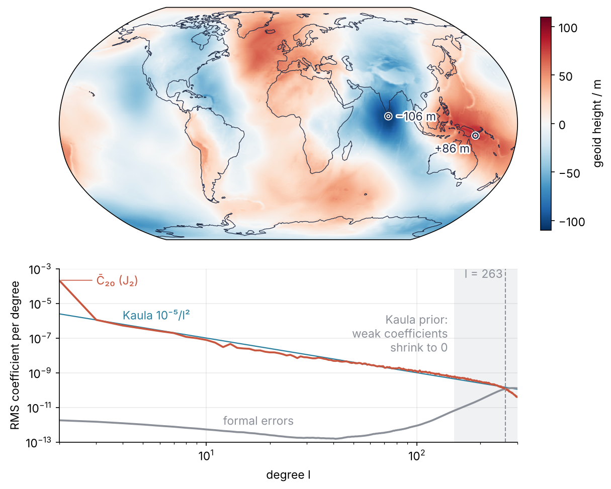
Top: geoid height in m relative to the WGS84 ellipsoid on a Robinson world map, from −106 m south of Sri Lanka to +86 m over New Guinea. Bottom: RMS coefficient per degree on log axes with Kaula's line and the formal errors, which overtake the signal at degree 263.

This is where we end up. On top is the geoid with the flattening taken away, a surface that departs from the ellipsoid by at most 106 m. Below it is the size of the coefficients per degree, which follows Kaula's line until the satellites' errors overtake the signal at degree 263. Step 6 draws it.

Setup

The model file is fetched once with pooch.retrieve, checked against the SHA-256 hash that pyshtools pins for it, and kept in pyshtools's cache, where pysh.datasets.Earth.GOCO06S() finds the same file. The URL is plain http, as pyshtools pins it; the hash is what makes that safe. The coastlines ship in assets/, as in Maps with Cartopy, and a download attempt by Cartopy stops the run.

import os
import warnings
from pathlib import Path

import numpy as np
import matplotlib.pyplot as plt
import matplotlib.patheffects as pe
warnings.filterwarnings("ignore", message="IProgress not found")  # a tqdm notice at import, not ours
import pooch
import pyshtools as pysh
import cartopy
import cartopy.crs as ccrs

cartopy.config["pre_existing_data_dir"] = Path("assets")       # holds shapefiles/natural_earth/physical/
warnings.simplefilter("error", cartopy.io.DownloadWarning)      # a download attempt stops the run

plt.rcParams.update({
    "figure.figsize": (8, 4.4), "figure.dpi": 110,
    "axes.spines.top": False, "axes.spines.right": False,
    "axes.grid": True, "grid.alpha": 0.25,
    "font.size": 11, "lines.linewidth": 1.8,
})
INK, ACCENT, SECOND, MUTED = "#1f2a44", "#c8553d", "#2a7f9e", "#8a8f98"

# WGS84 reference ellipsoid and rotation, used from Step 2 on
a = 6378137.0                 # m, equatorial radius
f = 1 / 298.257223563         # flattening
U0 = 62636851.7146            # m²/s², potential on the ellipsoid
OMEGA = 7.292115e-5           # rad/s

path = pooch.retrieve(
    "http://icgem.gfz-potsdam.de/getmodel/gfc/"
    "32ec2884630a02670476f752d2a2bf1c395d8c8d6d768090ed95b4f04b0d5863/GOCO06s.gfc",
    known_hash="sha256:351d9d20b84cd2c0f52ce77146b1e3b774f408200b579ffaf98593cf3d271819",
    path=pooch.os_cache("pyshtools"),
)
print(f"GOCO06s.gfc: {os.path.getsize(path):,} bytes ({os.path.getsize(path) / 1e6:.1f} MB)")

GOCO06s.gfc: 10,451,091 bytes (10.5 MB)

Step 1: Build one spherical harmonic by hand and expand it

Before the real model, one harmonic on its own. Every harmonic has a degree l and an order m. Its pattern has l nodal lines, circles on the sphere where it is zero, and m of them run through the poles: m = 0 is zonal, bands of latitude, and m = l is sectoral, wedges of longitude. pyshtools keeps the coefficients in an array coeffs[i, l, m], with i = 0 for the cosine terms C̄ₗₘ and i = 1 for the sine terms S̄ₗₘ.

The zonal harmonic of degree 2 is the Legendre polynomial P₂(sin φ) = (3 sin²φ − 1)/2 of the latitude φ, times √5. The √5 is the 4π normalization that the bar on C̄ marks: each harmonic is scaled so that its mean square over the sphere is 1. SHCoeffs.from_zeros makes a set of coefficients up to degree 20, all zero. Set one of them to Earth's C̄₂₀, let expand turn the coefficients into values on a grid of latitude and longitude, and compare with C̄₂₀ · √5 · P₂(sin φ):

C20 = -4.8416941e-4
coeffs = pysh.SHCoeffs.from_zeros(20, normalization="4pi")
coeffs.set_coeffs(C20, 2, 0)                    # value, degree l, order m
grid = coeffs.expand(grid="DH2")

phi = np.radians(grid.lats())
closed_form = C20 * np.sqrt(5) * (3 * np.sin(phi) ** 2 - 1) / 2
print(f"grid {grid.data.shape[0]} × {grid.data.shape[1]}")
print(f"pole {grid.data[0, 0]:.4e}   equator {grid.data[grid.nlat // 2, 0]:.4e}")
print(f"max difference to the closed form: {np.abs(grid.data - closed_form[:, None]).max():.1e}")

back = grid.expand()                            # and back to coefficients
others = back.coeffs.copy()
others[0, 2, 0] = 0
print(f"recovered C20 = {back.coeffs[0, 2, 0]:.8e}, largest other coefficient {np.abs(others).max():.1e}")

grid 43 × 85
pole -1.0826e-03   equator 5.4132e-04
max difference to the closed form: 6.5e-19
recovered C20 = -4.84169410e-04, largest other coefficient 4.4e-19

P₂ is 1 at the poles, so the pole value is √5 · C̄₂₀, the classical unnormalized coefficient C₂₀: −1.0826 × 10⁻³, the number from the opening with a minus sign. DH2 is the Driscoll-Healy grid of 2L+2 latitudes by 4L+4 longitudes, and expand adds the closing row and column by default (extend=True), hence 43 × 85. The grid matches the closed form, and the round trip returns C̄₂₀, to better than 10⁻¹⁸: grid and coefficients are the same field written two ways.

Step 2: Load the gravity model and read off J₂

Any .gfc file from ICGEM loads with one call, and lmax= would truncate it on reading. The file carries GM, the gravitational constant times Earth's mass, and r₀, the reference radius of the expansion, but not Earth's rotation rate, so you pass omega yourself. It matters from Step 4 on: the sea surface turns with Earth, so the potential that is constant on it is gravitation plus the centrifugal potential of the rotation, and omega supplies the second.

clm = pysh.SHGravCoeffs.from_file(path, format="icgem", errors="formal", omega=OMEGA)
print(f"GM = {clm.gm:.6e} m³/s²   r0 = {clm.r0:.1f} m   omega = {clm.omega:.6e} rad/s")
print(f"normalization {clm.normalization}, lmax {clm.lmax}, errors {clm.error_kind}")

J2 = -np.sqrt(5) * clm.coeffs[0, 2, 0]
print(f"J2 = {J2:.7e}")

GM = 3.986004e+14 m³/s²   r0 = 6378136.3 m   omega = 7.292115e-05 rad/s
normalization 4pi, lmax 300, errors formal
J2 = 1.0826357e-03

With Step 1 in hand this is one line: J₂ is minus the unnormalized C₂₀. Which coefficient comes next? Mask degree 0, degree 1 (zero in the file, because the origin is Earth's center of mass), and C̄₂₀, and look for the largest that remains:

rest = np.abs(clm.coeffs)
rest[:, :2, :] = 0
rest[0, 2, 0] = 0
i, l, m = np.unravel_index(rest.argmax(), rest.shape)
print(f"largest after C20: {'CS'[i]}({l},{m}) = {clm.coeffs[i, l, m]:.3e}, "
      f"|C20| is {abs(clm.coeffs[0, 2, 0]) / rest.max():.0f} times larger")

q = OMEGA**2 * clm.r0**3 / clm.gm               # centrifugal over gravitational acceleration
print(f"q = {q:.4e}   flattening (3 J2 + q)/2 = 1/{2 / (3 * J2 + q):.1f}   WGS84 1/{1 / f:.3f}")

largest after C20: C(2,2) = 2.439e-06, |C20| is 198 times larger
q = 3.4614e-03   flattening (3 J2 + q)/2 = 1/298.1   WGS84 1/298.257

It is C̄₂₂, sectoral and 198 times smaller: the equator itself is slightly elliptical. The last line checks the flattening. With q the ratio of centrifugal to gravitational acceleration at the equator, the first-order formula f ≈ (3J₂ + q)/2 gives 1/298.1 against 1/298.257 for WGS84. Rotation flattens the planet, and J₂ is that flattening seen from orbit.

Step 3: Plot the power spectrum against Kaula's rule

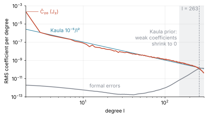
spectrum sums the squared coefficients of each degree, the power, and unit="per_lm" divides by the 2l+1 coefficients a degree has (S̄ₗ₀ is zero). The square root is the RMS coefficient per degree, the amplitude spectrum of the Fourier tutorial on the sphere. The method clm.spectrum() would return the geoid in m² per degree instead. Next to it go Kaula's rule, an empirical rule from the first satellite fields (Kaula 1966) that the RMS coefficient falls as 10⁻⁵/l², and the formal errors, the standard deviations the least-squares fit assigns each coefficient, "formal" because they trust the assumed noise.

The shaded band is a catch the file header states. GOCE, the satellite behind the short wavelengths, flew an orbit that does not cross the poles, and to bridge that gap GOCO06S is Kaula-regularized above degree 150. The regularization is a prior, an assumption added to the fit before it sees the data: each coefficient is zero, with Kaula's rule as its expected size. A coefficient the data pin down keeps its measured value, and one they barely constrain shrinks toward zero, not toward Kaula's line.

deg = np.arange(clm.lmax + 1)
rms = np.sqrt(pysh.spectralanalysis.spectrum(clm.coeffs, normalization="4pi", unit="per_lm"))
err = np.sqrt(pysh.spectralanalysis.spectrum(clm.errors, normalization="4pi", unit="per_lm"))
kaula = 1e-5 / np.maximum(deg, 1) ** 2
l_cross = deg[(deg >= 2) & (err > rms)][0]

def plot_spectrum(ax):
    l = deg[2:]
    ax.axvspan(150, 300, color=MUTED, alpha=0.12, lw=0)
    ax.text(140, 3e-6, "Kaula prior:\nweak coefficients\nshrink to 0", color=MUTED, va="top", ha="right")
    ax.loglog(l, kaula[2:], color=SECOND, lw=1.1)
    ax.loglog(l, err[2:], color=MUTED)
    ax.loglog(l, rms[2:], color=ACCENT)
    ax.axvline(l_cross, color=MUTED, ls="--", lw=1)
    ax.text(l_cross * 0.97, 3e-4, f"l = {l_cross}", color=MUTED, ha="right")
    ax.annotate("C̄₂₀ (J₂)", (2, rms[2]), (3, rms[2]), color=ACCENT, va="center",
                arrowprops=dict(arrowstyle="-", color=ACCENT, lw=0.8))
    ax.text(4, 1.2e-6, "Kaula 10⁻⁵/l²", color=SECOND)
    ax.text(12, 1e-12, "formal errors", color=MUTED)
    ax.set(xlabel="degree l", ylabel="RMS coefficient per degree", xlim=(2, 300), ylim=(1e-13, 1e-3))

fig, ax = plt.subplots(figsize=(7, 3.6))
plot_spectrum(ax)
plt.show()

print("  l   RMS/Kaula   error/RMS")
for L in [3, 10, 50, 100, 150, 200, 250, 263, 300]:
    print(f"{L:3d}   {rms[L] / kaula[L]:9.2f}   {err[L] / rms[L]:9.3f}")
band = rms[3:251] / kaula[3:251]
print(f"degrees 3 to 250: RMS/Kaula between {band.min():.2f} and {band.max():.2f}")
print(f"the errors exceed the signal from degree {l_cross}")

RMS coefficient per degree against degree l, log axes. The GOCO06S spectrum follows Kaula's line 1e-5/l² from degree 3 to about 250 and falls below it after the formal errors overtake the signal at degree 263; degree 2 sits far above.

  l   RMS/Kaula   error/RMS
  3        1.01       0.000
 10        0.78       0.000
 50        0.96       0.000
100        1.23       0.001
150        1.23       0.012
200        1.19       0.095
250        1.03       0.593
263        0.81       1.009
300        0.35       3.223
degrees 3 to 250: RMS/Kaula between 0.44 and 1.44
the errors exceed the signal from degree 263

Degree 2 sits far above the line, which is the flattening again. From degree 3 to 250 the spectrum stays between 0.44 and 1.44 of Kaula's rule while the RMS itself falls by nearly four orders of magnitude. Up to 250 the errors stay under 0.6 of the signal, so the data win over the prior. After 263 the errors pass the signal, the prior wins, and by degree 300 the spectrum has dropped to 0.35 of Kaula. That is where the satellites stop seeing, not where Earth becomes smooth.

Step 4: Map the geoid with and without the flattening

The geoid is the surface of constant gravity potential that the mean sea surface follows, here at the potential U0 of the WGS84 ellipsoid. clm.geoid(potref=U0) gives its height above the sphere of radius r₀:

geoid_sphere = clm.geoid(potref=U0).geoid
print(f"relative to the sphere: {geoid_sphere.data.min() / 1e3:.1f} km to {geoid_sphere.data.max():+.0f} m")

relative to the sphere: -21.4 km to +78 m

The −21 km is the flattening at the poles, and a sphere is the wrong reference. Pass the ellipsoid's a and f, and pyshtools measures the same surface from the WGS84 ellipsoid instead. Zeroing C̄₂₀ would not do that job: the flattening comes from J₂ and from the centrifugal potential together, as the formula of Step 2 says, and the ellipsoid accounts for both. Geodesists call the field of this rotating ellipsoid the normal field. The call returns an SHGeoid, whose .geoid is an SHGrid with lats(), lons(), and data:

geoid = clm.geoid(potref=U0, a=a, f=f).geoid
lats, lons, N = geoid.lats(), geoid.lons(), geoid.data
for name, k in [("min", N.argmin()), ("max", N.argmax())]:
    i, j = np.unravel_index(k, N.shape)
    print(f"{name} {N[i, j]:+7.1f} m at {lats[i]:+5.1f}° lat, {lons[j]:5.1f}° lon")

def geoid_map(ax, data, vlim):
    mesh = ax.pcolormesh(lons, lats, data, transform=ccrs.PlateCarree(),
                         cmap="RdBu_r", vmin=-vlim, vmax=vlim, rasterized=True)
    ax.coastlines(resolution="110m", color=INK, lw=0.6)
    ax.set_global()
    return mesh

def mark_extrema(ax, data):
    halo = [pe.withStroke(linewidth=3, foreground="white")]
    for k, dx, dy, ha, va in [(data.argmin(), 6, 0, "left", "center"), (data.argmax(), -4, -4, "right", "top")]:
        i, j = np.unravel_index(k, data.shape)
        ax.plot(lons[j], lats[i], "o", ms=5, mfc="none", mec=INK, mew=1.2, path_effects=halo,
                transform=ccrs.PlateCarree())
        ax.text(lons[j] + dx, lats[i] + dy, f"{data[i, j]:+.0f} m".replace("-", "−"), color=INK, ha=ha, va=va,
                path_effects=halo, transform=ccrs.PlateCarree())

fig = plt.figure(layout="compressed")
ax = fig.add_subplot(projection=ccrs.Robinson())
fig.colorbar(geoid_map(ax, N, 110), ax=ax, shrink=0.8, label="geoid height / m")
mark_extrema(ax, N)
plt.show()

min  -106.5 m at  +5.1° lat,  78.6° lon
max   +85.8 m at  -8.4° lat, 147.4° lon

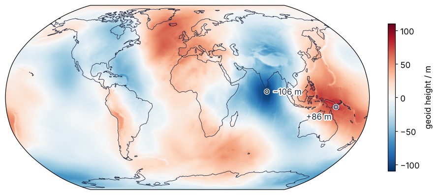
Geoid height in m relative to the WGS84 ellipsoid on a Robinson world map with coastlines. Lowest, −106 m, in the Indian Ocean south of Sri Lanka; highest, +86 m, over New Guinea, with a second high over the North Atlantic around Iceland.

Without the flattening the range shrinks from 21 km to 192 m. The deepest low, −106.5 m at 5.1°N 78.6°E, lies in the Indian Ocean south of Sri Lanka, and the highest point, +85.8 m at 8.4°S 147.4°E, over New Guinea. The North Atlantic around Iceland is the other high.

Step 5: Filter the field by degree

Cutting the sum off sharply at one degree is like stopping a Fourier series after N terms: the truncated sum overshoots and ripples around sharp features, the Gibbs ringing shown for images in MRI k-space reconstruction. A taper fades the last degrees out instead of cutting them. Here the weight w(l) is 1 up to degree 15, falls as a half cosine, and is 0 from degree 25:

w = np.clip((deg - 15) / 10, 0, 1)
w = 0.5 * (1 + np.cos(np.pi * w))               # 1 below l = 15, 0 above l = 25
low = clm.copy()
low.coeffs = clm.coeffs * w[None, :, None]
N_low = low.geoid(potref=U0, a=a, f=f).geoid.data
N_res = N - N_low
print(f"low-pass {N_low.min():+.1f} to {N_low.max():+.1f} m")
print(f"residual {N_res.min():+.1f} to {N_res.max():+.1f} m, standard deviation {N_res.std():.1f} m")

fig, axs = plt.subplots(2, 1, figsize=(8, 7.6), layout="compressed",
                        subplot_kw=dict(projection=ccrs.Robinson()))
for ax, data, vlim, label in [(axs[0], N_low, 110, "degrees ≤ 20 (tapered)"),
                              (axs[1], N_res, 25, "degrees above 20")]:
    fig.colorbar(geoid_map(ax, data, vlim), ax=ax, shrink=0.8, label="geoid height / m")
    ax.text(0.0, 1.02, label, transform=ax.transAxes, color=INK)
plt.show()

low-pass -104.2 to +77.0 m
residual -24.4 to +24.1 m, standard deviation 2.5 m

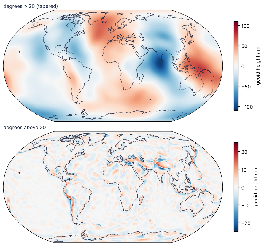
Two stacked Robinson maps of geoid height in m. Top: degrees up to about 20, tapered, from −104 m to +77 m, with the same broad lows and highs as the full geoid. Bottom: degrees above 20, ±24 m, tracing the trenches of Tonga-Kermadec, Japan, and Peru-Chile, the Andes, and the Himalaya.

The low-pass keeps nearly the whole range, −104 to +77 m: the broad lows and highs are degrees under 20, and they come from density differences deep in the mantle. The residual is small, ±24 m with a standard deviation of 2.5 m, and it draws the shallow structure: the subduction trenches of Tonga-Kermadec, Japan, and Peru-Chile, the Andes, the Himalaya. What a sharp cut does instead is in the Pitfalls.

Step 6: Put the geoid and the spectrum in one figure

The final figure stacks the map of Step 4 over the spectrum of Step 3, with the same functions and arrays:

fig = plt.figure(figsize=(8, 6.6), layout="constrained")
gs = fig.add_gridspec(2, 1, height_ratios=[4, 2.6])
ax_map = fig.add_subplot(gs[0], projection=ccrs.Robinson())
fig.colorbar(geoid_map(ax_map, N, 110), ax=ax_map, shrink=0.8, label="geoid height / m",
             ticks=[-100, -50, 0, 50, 100])
mark_extrema(ax_map, N)
plot_spectrum(fig.add_subplot(gs[1]))
plt.show()

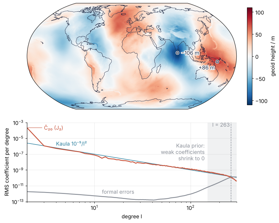
Top: geoid height in m relative to the WGS84 ellipsoid on a Robinson map, −106 m south of Sri Lanka to +86 m over New Guinea. Bottom: RMS coefficient per degree with Kaula's line and the formal errors, which cross the signal at degree 263.

Read together, every feature on the map is a sum of the harmonics counted below, and the harmonics past degree 263, with wavelengths under about 150 km, are more prior than measurement.

Pitfalls

Mixing normalizations. The symptom is a J₂ off by √5, or coefficients that match no paper. The cause is that the fields that use spherical harmonics have four conventions for the same harmonics, 4π, orthonormalized, Schmidt, and unnormalized, and some of them put the Condon-Shortley phase, a sign factor (−1)ᵐ, into the harmonics while others leave it out. Check clm.normalization and clm.csphase before you compare a number, and convert with clm.convert(normalization=..., csphase=...):

for norm in ["4pi", "ortho", "unnorm"]:
    print(f"{norm:6s}  C20 = {clm.convert(normalization=norm, lmax=2).coeffs[0, 2, 0]:.6e}")

4pi     C20 = -4.841694e-04
ortho   C20 = -1.716336e-03
unnorm  C20 = -1.082636e-03

The same coefficient differs by a factor of √(4π) = 3.5 between the first two.

Cutting sharply in degree. The symptom is ripples of a meter or two in a low-pass map that appear in neither the full field nor the tapered one. lmax_calc=20 is the tempting shortcut, and it is a box cutoff:

N_sharp = clm.geoid(potref=U0, a=a, f=f, lmax_calc=20).geoid.data
diff = N_sharp - N_low
i, j = np.unravel_index(np.abs(diff).argmax(), diff.shape)
print(f"sharp cut minus taper: up to {np.abs(diff).max():.2f} m at {lats[i]:+.1f}° lat, {lons[j]:.1f}° lon, "
      f"standard deviation {diff.std():.2f} m")

sharp cut minus taper: up to 1.94 m at +81.0° lat, 110.6° lon, standard deviation 0.52 m

Up to 1.94 m, with a standard deviation of 0.52 m over the grid. The fix is the taper of Step 5.

Loading an ICGEM file without omega. The symptom is a geoid kilometers away from the ellipsoid, with no warning. A .gfc file carries GM and r₀ but no rotation rate, so from_file leaves omega as None, and geoid silently leaves out the centrifugal potential:

no_omega = pysh.SHGravCoeffs.from_file(path, format="icgem", errors="formal")
print(f"omega = {no_omega.omega}, geoid minimum {no_omega.geoid(potref=U0, a=a, f=f).geoid.data.min() / 1e3:.1f} km")

omega = None, geoid minimum -11.1 km

Pass omega= on loading, or set clm.omega afterwards.

Variations

Mars and its dichotomy. pysh.datasets.Mars.MOLA_shape(lmax=...) loads the shape of Mars, whose degree-1 term carries the dichotomy between the low northern plains and the southern highlands. Only the smallest of its four files that covers lmax is downloaded, so ask for a low degree first.
The Moon's gravity. pysh.datasets.Moon.GRGM1200B(lmax=...) goes to degree 1200, with a Kaula constraint above 600, and shows the mascons of the large impact basins.
Gravity anomalies instead of the geoid. clm.expand(a=a, f=f) returns gravity on the ellipsoid, with .rad and .total grids. Its spectrum falls more slowly than the geoid's, so the filter of Step 5 matters more.
A field from scattered measurements. pysh.SHCoeffs.from_least_squares(data, lat, lon, lmax) fits coefficients to values at arbitrary points.

Cheat sheet

clm = pysh.SHGravCoeffs.from_file(fn, format="icgem", errors="formal", omega=OMEGA)  # any ICGEM .gfc
clm.coeffs[i, l, m]                                    # i = 0 cosine C̄lm, i = 1 sine S̄lm
J2 = -np.sqrt(5) * clm.coeffs[0, 2, 0]                 # 4π-normalized C̄20 to J2
rms = np.sqrt(pysh.spectralanalysis.spectrum(clm.coeffs, unit="per_lm"))  # RMS coefficient per degree
N = clm.geoid(potref=U0, a=a, f=f).geoid.data          # geoid height above the ellipsoid, m
clm.geoid(potref=U0, a=a, f=f, lmax_calc=20)           # sharp cut: rings
low.coeffs = clm.coeffs * w[None, :, None]             # tapered filter, w(l) from 1 to 0
grid = pysh.SHCoeffs.from_zeros(20).expand(); grid.expand()  # coefficients to grid and back
clm.convert(normalization="ortho", csphase=-1)         # other conventions