Hückel theory with SymPy: exact orbital energies of butadiene and benzene

The problem: how much does delocalization stabilize butadiene and benzene?

Butadiene is drawn with two double bonds, and chemistry courses say that they talk to each other. Benzene is said to be unusually stable. Hückel theory turns both statements into numbers, and SymPy computes them exactly: the four π electrons of butadiene are bound 0.472β more strongly than those of two separate ethylenes, and the six of benzene gain 2β over three ethylenes. Here β, the resonance integral, is an energy and is negative.

Each carbon contributes one p orbital to the π system, and the Hückel Hamiltonian has one row per carbon. The diagonal holds the Coulomb integral α, the energy of an electron in a lone p orbital; β stands wherever two carbons are bonded, and every other entry is zero. Only neighbors interact and the overlap of the orbitals is neglected; Atkins derives the matrix from the variational principle. For butadiene, with the carbons numbered along the chain,

Its eigenvalues are the orbital energies \(E = \alpha + \lambda\beta\), with \(\lambda = \pm 1.618\) and \(\pm 0.618\), the golden ratio and its inverse. Four electrons fill the two bonding orbitals and give \(E_\pi = 4\alpha + 2\sqrt5\,\beta = 4\alpha + 4.472\beta\), against \(4\alpha + 4\beta\) for two ethylenes.

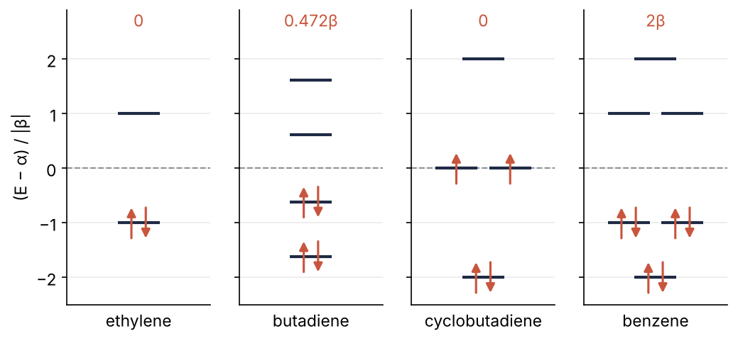
Each level is an exact eigenvalue from SymPy's linear algebra, each arrow an electron, and the number above each molecule its delocalization energy; Step 6 draws the figure. Benzene's six electrons close a shell and cyclobutadiene's four do not, and Step 5 proves why for every ring.

Setup

One cell: SymPy, the plotting style, the symbols, and two helpers that write a molecule as a list of bonds between numbered carbons.

import sympy as sp
import matplotlib.pyplot as plt

plt.rcParams.update({
    "figure.figsize": (8, 3.6), "figure.dpi": 110,
    "axes.spines.top": False, "axes.spines.right": False,
    "axes.grid": True, "grid.alpha": 0.25,
    "font.size": 11, "lines.linewidth": 1.8,
})
INK, ACCENT, SECOND, MUTED = "#1f2a44", "#c8553d", "#2a7f9e", "#8a8f98"

alpha, beta, E = sp.symbols("alpha beta E")      # no sign assumption on beta (Pitfall 1)
lam = sp.Symbol("lambda")                       # eigenvalue of the adjacency matrix: E = alpha + lam*beta

def chain(n):
    return [(i, i + 1) for i in range(n - 1)]

def ring(n):
    return chain(n) + [(n - 1, 0)]

print("butadiene bonds:", chain(4))

butadiene bonds: [(0, 1), (1, 2), (2, 3)]

Step 1: Build the Hückel matrix from a bond list

The matrix starts as α times the identity and gets β at both \((i, j)\) and \((j, i)\) for every bond, so it is symmetric by construction:

def huckel(n, bonds):
    M = alpha * sp.eye(n)
    for i, j in bonds:
        M[i, j] = M[j, i] = beta
    return M

def adjacency(n, bonds):
    return huckel(n, bonds).subs({alpha: 0, beta: 1})

H = huckel(4, chain(4))
A = adjacency(4, chain(4))
sp.pprint(H)
sp.pprint(A)

⎡α  β  0  0⎤
⎢          ⎥
⎢β  α  β  0⎥
⎢          ⎥
⎢0  β  α  β⎥
⎢          ⎥
⎣0  0  β  α⎦
⎡0  1  0  0⎤
⎢          ⎥
⎢1  0  1  0⎥
⎢          ⎥
⎢0  1  0  1⎥
⎢          ⎥
⎣0  0  1  0⎦

Setting α = 0 and β = 1 leaves the adjacency matrix \(A\) of the carbon skeleton, a 1 for every bond. So \(H = \alpha\mathbf 1 + \beta A\): the identity shifts every eigenvalue by α and β scales them, so the eigenvalues of \(H\) are \(E = \alpha + \lambda\beta\), with λ an eigenvalue of \(A\). Every result below is a statement about \(A\), the same matrix that describes a network in The graph Laplacian: why its second eigenvector cuts a network in two.

Step 2: Turn the secular determinant into a polynomial with charpoly and factor

An eigenvalue \(E\) of \(H\) is a number that makes \(H - E\mathbf 1\) singular, as in Eigenvalues with numpy.linalg: normal modes of coupled oscillators, so the eigenvalues are the roots of \(\det(E\mathbf 1 - H)\), the secular determinant of the chemistry textbooks. charpoly computes it as a polynomial object, which .as_expr() turns into an ordinary expression for subs:

p_E = H.charpoly(E).as_expr()
print(p_E)

E**4 - 4*E**3*alpha + E**2*(6*alpha**2 - 3*beta**2) + E*(-4*alpha**3 + 6*alpha*beta**2) + alpha**4 - 3*alpha**2*beta**2 + beta**4

A quartic with α and β in every coefficient. Substitute \(E = \alpha + \lambda\beta\) and divide by \(\beta^4\), since \(\det(\lambda\beta\mathbf 1 - \beta A) = \beta^4\det(\lambda\mathbf 1 - A)\), and the polynomial of \(A\) appears. The expand and factor are the rewrites from SymPy from the ground up: where the pendulum's 1.74 % comes from:

p = sp.expand(p_E.subs(E, alpha + lam * beta) / beta**4)
print(p)
print(sp.factor(p))
print("A.charpoly(lam) minus p:", A.charpoly(lam).as_expr() - p)

lambda**4 - 3*lambda**2 + 1
(lambda**2 - lambda - 1)*(lambda**2 + lambda - 1)
A.charpoly(lam) minus p: 0

Two quadratics, and A.charpoly(lam) gives the same polynomial in one call. eigenvals returns a dictionary from eigenvalue to multiplicity, in no useful order. The λ are numbers and sort by float. An energy of H still holds α and β, which float cannot evaluate, so its sort key sets α = 0 and β = −1: that is \((E - \alpha)/|\beta|\) for a negative β, and the most bonding orbital comes first (Pitfall 1 explains the sign):

levels = A.eigenvals()
for l in sorted(levels, key=float, reverse=True):
    print(f"λ = {str(l):16s} = {float(l):7.4f}   multiplicity {levels[l]}")

E_levels = sorted(H.eigenvals(), key=lambda e: float(e.subs({alpha: 0, beta: -1})))
print(E_levels[0])

λ = 1/2 + sqrt(5)/2  =  1.6180   multiplicity 1
λ = -1/2 + sqrt(5)/2 =  0.6180   multiplicity 1
λ = 1/2 - sqrt(5)/2  = -0.6180   multiplicity 1
λ = -sqrt(5)/2 - 1/2 = -1.6180   multiplicity 1
alpha + beta/2 + sqrt(5)*beta/2

The roots are \((1 \pm \sqrt5)/2\) and \((-1 \pm \sqrt5)/2\), that is ±1.618 and ±0.618, and H.eigenvals() gives the most bonding orbital as \(E = \alpha + 1.618\beta\). Factor first anyway. It shows the structure, two quadratics, that eigenvals buries in radicals. It also splits the polynomial over the rationals into factors of degree four or less, whose roots can always be written in radicals, and larger irreducible ones, whose roots in general cannot (Pitfall 3).

Step 3: Fill the orbitals and get the total π energy

With β < 0, \(E = \alpha + \lambda\beta\) is lowest for the largest λ, so the bonding orbitals are those with λ > 0 and filling starts at the top of the λ list. The function below expands each λ by its multiplicity and puts two electrons into each orbital until they run out, one into the last if the count is odd:

def occupy(levels, n_electrons):
    """(lambda, electrons) for every orbital, most bonding first."""
    orbitals = [l for l in sorted(levels, key=float, reverse=True) for _ in range(levels[l])]
    filled = []
    for l in orbitals:
        n = min(2, n_electrons)
        filled.append((l, n))
        n_electrons -= n
    return filled

def pi_energy(n_carbons, filled):
    return n_carbons * alpha + sp.simplify(sum(n * l for l, n in filled)) * beta

for name, n, bonds, n_el in [("ethylene", 2, chain(2), 2), ("butadiene", 4, chain(4), 4),
                             ("allyl", 3, chain(3), 3)]:
    filled = occupy(adjacency(n, bonds).eigenvals(), n_el)
    occupied = [(str(l), n_e) for l, n_e in filled if n_e > 0]
    print(f"{name:10s} E_pi = {str(pi_energy(n, filled)):28s} filled (lambda, electrons): {occupied}")

ethylene   E_pi = 2*alpha + 2*beta             filled (lambda, electrons): [('1', 2)]
butadiene  E_pi = 4*alpha + 2*sqrt(5)*beta     filled (lambda, electrons): [('1/2 + sqrt(5)/2', 2), ('-1/2 + sqrt(5)/2', 2)]
allyl      E_pi = 3*alpha + 2*sqrt(2)*beta     filled (lambda, electrons): [('sqrt(2)', 2), ('0', 1)]

Ethylene puts both electrons into λ = 1, butadiene gets \(4\alpha + 2\sqrt5\,\beta\), and the allyl radical, three carbons and three electrons, leaves the odd electron alone in the nonbonding level λ = 0, where it adds nothing to \(E_\pi = 3\alpha + 2\sqrt2\,\beta\).

The delocalization energy is what \(E_\pi\) gains over the same electrons in isolated double bonds: \(E_\pi - N\alpha - 2\beta\,n_{\mathrm{C=C}}\), with \(N\) the number of carbons and \(n_{\mathrm{C=C}}\) the double bonds in one Kekulé structure. The allyl radical gets none: its reference, a double bond plus a lone electron, needs a convention of its own. For butadiene:

E_pi = pi_energy(4, occupy(levels, 4))
deloc = sp.simplify((E_pi - 4 * alpha - 2 * 2 * beta) / beta)
print(f"delocalization = ({deloc}) beta = {float(deloc):.4f} beta")

delocalization = (-4 + 2*sqrt(5)) beta = 0.4721 beta

That is \((2\sqrt5 - 4)\beta = 0.472\beta\), 12 % more than the 4β of two ethylenes.

Step 4: Get the orbitals from eigenvects and compute bond orders

eigenvects returns a list of triples: an eigenvalue, its multiplicity, and a list of eigenvectors. Straight out of SymPy a vector is neither simplified nor normalized:

eig = sorted(H.eigenvects(), key=lambda t: float(t[0].subs({alpha: 0, beta: -1})))
value, mult, vectors = eig[0]
print(value)
print(vectors[0].T)

alpha + beta/2 + sqrt(5)*beta/2
Matrix([[1, -alpha/beta + (alpha + beta/2 + sqrt(5)*beta/2)/beta, -alpha/beta + (alpha + beta/2 + sqrt(5)*beta/2)/beta, 1]])

The α/β terms cancel once each entry is simplified, which applyfunc(sp.simplify) does; dividing by norm() gives a unit vector, and one more simplify tidies the result:

orbitals = []
for value, mult, vectors in eig:
    v = vectors[0].applyfunc(sp.simplify)
    orbitals.append((v / v.norm()).applyfunc(sp.simplify))

print(orbitals[0].T)
print("as numbers:", [round(float(c), 3) for c in orbitals[0]])

Matrix([[1/sqrt(sqrt(5) + 5), (1 + sqrt(5))/(2*sqrt(sqrt(5) + 5)), (1 + sqrt(5))/(2*sqrt(sqrt(5) + 5)), 1/sqrt(sqrt(5) + 5)]])
as numbers: [0.372, 0.602, 0.602, 0.372]

All four coefficients of the most bonding orbital have the same sign, 0.372 on the end carbons and 0.602 in the middle.

The product \(c_r c_s\) of one orbital is positive when the orbital has the same sign on the bonded atoms \(r\) and \(s\), bonding between them, and negative when the signs differ. Summed over the electrons, Coulson's π bond order

with \(n_k\) the electrons in orbital \(k\), counts net bonding electron pairs between the two atoms, the same bookkeeping as (bonding − antibonding)/2 for a diatomic. Ethylene's filled orbital \((1, 1)/\sqrt2\) gives \(p = 1\), a full π bond, and the total bond order adds the σ bond, \(1 + p\). For a column vector c, c * c.T is the outer product, np.outer in NumPy, so the whole matrix is one sum over orbitals zipped with Step 3's occupy, both most bonding first:

P = sum((n_k * c * c.T for c, (_, n_k) in zip(orbitals, occupy(levels, 4))), sp.zeros(4)).applyfunc(sp.simplify)
for r, s in [(0, 1), (1, 2)]:
    print(f"p_{r + 1}{s + 1} = {str(P[r, s]):10s} = {float(P[r, s]):.3f}   total order {1 + float(P[r, s]):.3f}")
print("pi electrons per carbon:", [P[i, i] for i in range(4)])

p_12 = 2*sqrt(5)/5 = 0.894   total order 1.894
p_23 = sqrt(5)/5  = 0.447   total order 1.447
pi electrons per carbon: [1, 1, 1, 1]

The terminal bonds have total order 1.894, less than double, and the central bond 1.447, well above single. That is the talking, in numbers. The diagonal of \(P\) is exactly 1 on every carbon, so the π charges are zero; this holds for every molecule in this tutorial and changes with a heteroatom (Variations).

Step 5: Prove the ring energies 2cos(2πk/N) and the 4n + 2 rule

A ring of \(N\) equal carbons looks the same after every atom moves one place around. That move is a matrix \(R\), and since it keeps every bond, \(RA = AR\). So \(R\) turns an orbital of energy λ into one of the same λ, and within each level, like any square matrix, it has eigenvectors, complex if need be: orbitals that the move only multiplies by a number ω. Then \(c_j = \omega^j c_0\), and after \(N\) steps the orbital is back: \(\omega^N = 1\). The \(N\) choices are \(\omega_k = e^{2\pi i k/N}\) for \(k = 0, \dots, N-1\). Row \(j\) of \(A\) has ones at \(j \pm 1\), around the ring; apply it and divide by \(c_j\):

N = sp.Symbol("N", integer=True, positive=True)
j, k = sp.symbols("j k", integer=True)
omega = sp.exp(2 * sp.pi * sp.I * k / N)

lam_k = sp.simplify((omega**(j - 1) + omega**(j + 1)) / omega**j)
print(lam_k.rewrite(sp.cos))

2*cos(2*pi*k/N)

The ratio does not depend on \(j\), so every \(\omega_k\) gives an orbital with \(\lambda_k = 2\cos(2\pi k/N)\), for all \(N\) at once. There are no others: the overlap \(\langle k | k' \rangle = \sum_j \omega_k^{-j}\omega_{k'}^{j}\), with the left vector conjugated, is a geometric sum that vanishes unless \(k = k'\), and \(N\) orthogonal vectors in \(N\) dimensions leave no room for another. A check against eigenvals, and benzene's overlap with V.H, the conjugate transpose:

for n in [3, 4, 5, 6, 8]:
    formula = {}
    for kk in range(n):
        l = sp.simplify(2 * sp.cos(2 * sp.pi * kk / n))
        formula[l] = formula.get(l, 0) + 1
    print(f"N = {n}:", adjacency(n, ring(n)).eigenvals() == formula,
          sorted(formula.items(), key=lambda t: -float(t[0])))

V = sp.Matrix(6, 6, lambda jj, kk: sp.exp(2 * sp.pi * sp.I * jj * kk / 6))
sp.pprint((V.H * V).applyfunc(lambda e: sp.simplify(sp.expand_complex(e))))

N = 3: True [(2, 1), (-1, 2)]
N = 4: True [(2, 1), (0, 2), (-2, 1)]
N = 5: True [(2, 1), (-1/2 + sqrt(5)/2, 2), (-sqrt(5)/2 - 1/2, 2)]
N = 6: True [(2, 1), (1, 2), (-1, 2), (-2, 1)]
N = 8: True [(2, 1), (sqrt(2), 2), (0, 2), (-sqrt(2), 2), (-2, 1)]
⎡6  0  0  0  0  0⎤
⎢                ⎥
⎢0  6  0  0  0  0⎥
⎢                ⎥
⎢0  0  6  0  0  0⎥
⎢                ⎥
⎢0  0  0  6  0  0⎥
⎢                ⎥
⎢0  0  0  0  6  0⎥
⎢                ⎥
⎣0  0  0  0  0  6⎦

The overlap is 6 times the identity. The conjugates \(\omega_k^j\) and \(\omega_{N-k}^j\) share a λ, and their sum and difference are the textbooks' real cosine and sine orbitals.

The level \(k = 0\) is single, at λ = 2; for even \(N\), so is \(k = N/2\), at λ = −2 and empty. Every other \(k\) pairs with \(N - k\). Filling from λ = 2 down, a shell closes after 2, 6, 10, … electrons, \(4n + 2\): benzene's six close it; cyclobutadiene's four and cyclooctatetraene's eight leave two electrons in a pair that holds four.

Step 6: Compare the four molecules in one diagram

Step 3's occupy fills one orbital after another, so two electrons left for a degenerate pair both land in its first orbital. The version below spreads them one per orbital first (Hund's rule). \(E_\pi\) stays the same; only cyclobutadiene's arrows change:

def occupy(levels, n_electrons):
    """(lambda, electrons) for every orbital, most bonding first; Hund's rule within a level."""
    filled = []
    for l in sorted(levels, key=float, reverse=True):
        m = levels[l]
        n = min(2 * m, n_electrons)
        n_electrons -= n
        filled += [(l, n // m + (i < n % m)) for i in range(m)]   # the first n % m orbitals get one more
    return filled

molecules = {"ethylene": (2, chain(2)), "butadiene": (4, chain(4)),
             "cyclobutadiene": (4, ring(4)), "benzene": (6, ring(6))}
double_bonds = {"ethylene": 1, "butadiene": 2, "cyclobutadiene": 2, "benzene": 3}   # one Kekulé structure

deloc = {}
for name, (n, bonds) in molecules.items():
    filled = occupy(adjacency(n, bonds).eigenvals(), n)
    e = sp.simplify(sum(n_e * l for l, n_e in filled))
    deloc[name] = sp.simplify(e - 2 * double_bonds[name])
    print(f"{name:15s} E_pi - N alpha = ({str(e):9s}) beta   "
          f"delocalization = ({str(deloc[name]):14s}) beta = {float(deloc[name]):.3f} beta")

ethylene        E_pi - N alpha = (2        ) beta   delocalization = (0             ) beta = 0.000 beta
butadiene       E_pi - N alpha = (2*sqrt(5)) beta   delocalization = (-4 + 2*sqrt(5)) beta = 0.472 beta
cyclobutadiene  E_pi - N alpha = (4        ) beta   delocalization = (0             ) beta = 0.000 beta
benzene         E_pi - N alpha = (8        ) beta   delocalization = (2             ) beta = 2.000 beta

Copy

def draw_levels(ax, n, bonds, ink, accent, lw=2.0, arrow_lw=1.5, head=12):
    filled = occupy(adjacency(n, bonds).eigenvals(), n)
    lams = [l for l, _ in filled]
    for idx, (l, n_el) in enumerate(filled):
        m, i = lams.count(l), lams[:idx].count(l)     # position inside a degenerate set
        x, y = (i - (m - 1) / 2) * 0.9, -float(l)      # bonding (lambda > 0) at the bottom, since beta < 0
        ax.plot([x - 0.35, x + 0.35], [y, y], color=ink, lw=lw, solid_capstyle="butt")
        spins = [(0, 1)] if n_el == 1 else [(-0.12, 1), (0.12, -1)][:n_el]
        for dx, up in spins:
            ax.annotate("", xy=(x + dx, y + 0.28 * up), xytext=(x + dx, y - 0.28 * up),
                        arrowprops=dict(arrowstyle="-|>", color=accent, lw=arrow_lw, mutation_scale=head,
                                        shrinkA=0, shrinkB=0))

fig, axes = plt.subplots(1, 4, sharey=True)
for ax, (name, (n, bonds)) in zip(axes, molecules.items()):
    ax.axhline(0, color=MUTED, lw=1, ls="--")
    draw_levels(ax, n, bonds, INK, ACCENT)
    label = f"{float(deloc[name]):.3g}β" if deloc[name] != 0 else "0"   # delocalization energy
    ax.text(0, 2.6, label, color=ACCENT, ha="center")
    ax.set(xlim=(-1.2, 1.2), ylim=(-2.5, 2.9), xticks=[], xlabel=name)
axes[0].set(yticks=[-2, -1, 0, 1, 2], ylabel="(E − α) / |β|")
plt.show()

Benzene's three filled levels give 8β against 6β for three ethylenes. Cyclobutadiene gains nothing and is left with an open shell, the antiaromatic case of Hückel theory; the real molecule escapes it by distorting to a rectangle.

Pitfalls

The sign of β. Symptom: the "lowest" orbitals come out antibonding, and butadiene's \(E_\pi\) reads \(4\alpha - 4.472\beta\). Cause: the λ list was sorted ascending, as if β were positive, while β is negative and \(E = \alpha + \lambda\beta\) falls as λ rises. Fix: sort by λ descending, as occupy does, or substitute a negative β before sorting energies, as Steps 2 and 4 do. Declaring sp.Symbol("beta", negative=True) would not spare you that substitution, because float still cannot evaluate an energy that contains α. That is why the symbols here carry no assumptions. The textbook variable flips the sign too: many texts write the secular polynomial in \(x = (\alpha - E)/\beta\), which is \(-\lambda\), so convert a root read off a textbook by λ = −x. For the chains and even rings here the roots come in ± pairs and the two lists agree, which hides the trap. The seven-membered ring of Pitfall 3 does not: its λ = 2 is x = −2.

Degenerate levels from eigenvects. For a degenerate eigenvalue, such as benzene's λ = ±1, eigenvects returns some basis of the eigenspace, and its vectors are not orthogonal to each other. Normalizing each one, as in Step 4, is then not enough:

eig6 = sorted(adjacency(6, ring(6)).eigenvects(), key=lambda t: float(t[0]), reverse=True)
occupied = eig6[:2]                                        # lambda = 2 and the pair at lambda = 1

def bond_orders(vectors):
    P6 = sum((2 * c * c.T for c in vectors), sp.zeros(6)).applyfunc(sp.simplify)
    return [P6[i, (i + 1) % 6] for i in range(6)], [P6[i, i] for i in range(6)]

naive = [v / v.norm() for _, _, vs in occupied for v in vs]
fixed = [v for _, _, vs in occupied for v in sp.GramSchmidt(vs, orthonormal=True)]
print("normalized only:", *bond_orders(naive))
print("GramSchmidt:    ", *bond_orders(fixed))

normalized only: [5/6, 1/3, 5/6, 5/6, 1/3, 5/6] [4/3, 5/6, 5/6, 4/3, 5/6, 5/6]
GramSchmidt:     [2/3, 2/3, 2/3, 2/3, 2/3, 2/3] [1, 1, 1, 1, 1, 1]

Six identical bonds with orders 5/6 and 1/3, and π populations of 4/3 and 5/6, is the symptom. sp.GramSchmidt(vectors, orthonormal=True) on each degenerate set makes every bond 2/3 and every population 1. \(P\) is the same for every orthonormal basis of the pair, so the bond orders are well defined.

Past degree four. Symptom: eigenvals for the seven-membered ring returns three of its eigenvalues as long expressions with cube roots of complex numbers, although the eigenvalues of a real symmetric matrix are real. A cubic with three real irrational roots can be written in radicals only by passing through complex numbers. For larger irreducible polynomials, eigenvals gives CRootOf(poly, k), SymPy's exact placeholder for "the k-th root of this polynomial", which has a value to any precision but no formula. Fix: factor first, keep what factors exactly, and get the rest from nroots. The cell prints the longest eigenvalue, measured by count_ops, then the factored polynomial and the cubic's roots:

A7 = adjacency(7, ring(7))
print(max(A7.eigenvals(), key=lambda l: sp.count_ops(l)))
p7 = sp.factor(A7.charpoly(lam).as_expr())
print(p7)
cubic = [f for f, m in sp.factor_list(p7)[1] if sp.degree(f, lam) == 3][0]
print(sp.Poly(cubic, lam).nroots(n=4))

-1/3 + (-1/2 - sqrt(3)*I/2)*(7/54 + 7*sqrt(3)*I/18)**(1/3) + 7/(9*(-1/2 - sqrt(3)*I/2)*(7/54 + 7*sqrt(3)*I/18)**(1/3))
(lambda - 2)*(lambda**3 + lambda**2 - 2*lambda - 1)**2
[-1.802, -0.4450, 1.247]

λ = 2 once and the cubic's three roots twice each: −1.802, −0.445, and 1.247, which are \(2\cos(2\pi k/7)\) for \(k = 3, 2, 1\). When you report them, say that these three are numerical.

Variations

• A heteroatom: pyridine. Put \(\alpha + h\beta\) on one diagonal entry of the benzene ring, so \(A\) gets \(h\) there. A.charpoly(lam) factors into \((\lambda - 1)(\lambda + 1)\) and a quartic in λ and \(h\). Substitute \(\lambda = 2 + c_1 h + c_2 h^2\) into the quartic, take series in \(h\) as in Perturbation theory with SymPy: the Duffing oscillator's frequency shift, and solve each order: the lowest level moves to \(\lambda = 2 + h/6 + 35h^2/432\). The diagonal of \(P\) is no longer 1, and the charges become the result.
• Naphthalene. Ten carbons, eleven bonds. factor splits the degree-10 polynomial into \((\lambda - 1)(\lambda + 1)(\lambda^2 \pm \lambda - 1)(\lambda^2 \pm \lambda - 3)\), so every root stays readable, and the delocalization energy is \((2\sqrt5 + 2\sqrt{13} - 8)\beta = 3.683\beta\).
• The long-chain limit. A chain of \(N\) carbons has \(\lambda_k = 2\cos(k\pi/(N + 1))\); the proof is Step 5's with \(c_j = \sin(jk\pi/(N + 1))\), a standing wave like the particle in a box. The gap between the highest filled and lowest empty level, \(4\sin(\pi/(2(N + 1)))\,|\beta|\), is \(1.236|\beta|\) for butadiene and \(0.299|\beta|\) for twenty carbons, the reason long polyenes absorb visible light.
• Graphene. On the honeycomb lattice the orbital repeats from cell to cell up to a phase, which gives \(E = \alpha \pm \beta\,|1 + e^{i\mathbf k\cdot\mathbf a_1} + e^{i\mathbf k\cdot\mathbf a_2}|\), the Hückel model of graphene's π band. lambdify it and draw it over the wave vectors of one cell, as in Band structure with plane waves in NumPy: an electron in a 1D crystal.

Cheat sheet

H = alpha * sp.eye(n)                                      # Hückel matrix from a bond list
for i, j in bonds: H[i, j] = H[j, i] = beta
A = H.subs({alpha: 0, beta: 1})                            # E = alpha + lam*beta, lam eigenvalue of A
sp.factor(A.charpoly(lam).as_expr())                       # same as H.charpoly(E) with E = alpha + lam*beta
A.eigenvals()                                              # {lam: multiplicity}; sort by float, largest = most bonding
eig = sorted(A.eigenvects(), key=lambda t: float(t[0]), reverse=True)   # (lam, mult, vectors) per level
v = eig[0][2][0].applyfunc(sp.simplify); v = v / v.norm()  # vectors come unsimplified, unnormalized
occupied = [c for _, _, vs in eig[:2] for c in sp.GramSchmidt(vs, orthonormal=True)]   # filled levels, degenerate ones orthonormalized
P = sum((2 * c * c.T for c in occupied), sp.zeros(n))      # closed shell; bond orders off the diagonal, pi charges on it
sp.Poly(irreducible_part, lam).nroots()                    # numerical roots past degree four

Further reading

• SymPy documentation: Matrices, for eigenvals, eigenvects, charpoly, and GramSchmidt.
• P. Atkins and J. de Paula, Physical Chemistry, the section on the Hückel approximation, for the variational derivation of the secular determinant and the textbook diagrams.
• A. Streitwieser, Molecular Orbital Theory for Organic Chemists (Wiley, 1961), for bond orders, charges, and heteroatom parameters.
• Related tutorials on this site: SymPy from the ground up: where the pendulum's 1.74 % comes from, Eigenvalues with numpy.linalg: normal modes of coupled oscillators, Von Neumann stability analysis with SymPy: the leapfrog Courant limit, Computer algebra: formulas as trees, exact until you ask for digits, The graph Laplacian: why its second eigenvector cuts a network in two, Band structure with plane waves in NumPy: an electron in a 1D crystal.
• Download the notebook. It was executed with the library versions in the header.