Voronoi and Delaunay: the rainfall over a catchment from twelve gauges
Afterwards you can say what Voronoi cells and Delaunay triangles are, why each is the other's dual, and weight uneven measurements by cell area.
- Field
- Biology, Engineering, Geology
- Prerequisites
- none beyond Python basics
- Libraries
matplotlib 3.11.2numpy 2.4.3scipy 1.18.1shapely 2.2.0
py-voronoi-delaunay.ipynb, executed with the versions above. The download needs a free account
Run it yourself. In a terminal, this installs exactly the versions above:
pip install numpy==2.4.3 scipy==1.18.1 shapely==2.2.0 matplotlib==3.11.2 jupyterlabThe question
Here are twelve rain gauges in a river catchment of about 309 km², with the totals they recorded during one storm. A hydrologist wants one number from them, the mean rainfall over the whole catchment, because that is what the river will have to carry away. Getting it right takes two pieces of geometry that turn up wherever measurements are scattered over an area: the Voronoi diagram and the Delaunay triangulation.
Show code
import numpy as np
import matplotlib.pyplot as plt
from matplotlib.path import Path
from matplotlib.colors import LinearSegmentedColormap
from matplotlib.patheffects import withStroke

plt.rcParams.update({
    "figure.figsize": (7, 4.8), "figure.dpi": 110,
    "axes.spines.top": False, "axes.spines.right": False,
    "axes.grid": True, "grid.alpha": 0.25,
    "font.size": 11, "lines.linewidth": 1.8,
})
INK, ACCENT, SECOND, MUTED = "#1f2a44", "#c8553d", "#2a7f9e", "#8a8f98"
RAIN = LinearSegmentedColormap.from_list("rain", ["#ffffff", SECOND])   # one hue, light to dark

# The catchment, the gauges, and the rain are synthetic, so that the answer can be
# checked at the end. Pretend you have not seen this cell.
catchment = np.array([                                    # outline in local plane coordinates, km
    (0.5, 2.5), (4.5, 0.3), (9.0, 0.8), (13.5, 0.0), (18.0, 1.5), (22.0, 3.0), (24.0, 7.0),
    (23.5, 12.0), (21.0, 15.5), (16.5, 17.0), (11.5, 16.5), (7.0, 14.0), (3.0, 11.5), (0.0, 7.0),
])
outline = Path(catchment)
x, y = catchment.T
area = 0.5 * abs(x @ np.roll(y, -1) - y @ np.roll(x, -1))   # shoelace formula
town = np.array([4.5, 4.0])

def rain(x, y):
    """Storm total in mm: rising from the south-west toward the ridge, plus one storm cell."""
    ridge = 20 + 35 * (0.6 * (x - 0.5) / 23.5 + 0.4 * y / 17.0)
    cell = 12 * np.exp(-((x - 13) ** 2 + (y - 9) ** 2) / (2 * 3.5 ** 2))
    return ridge + cell

rng = np.random.default_rng(1911)
gauges = []
while len(gauges) < 5:                                    # five by the town, where the observers live
    p = town + 1.2 * rng.standard_normal(2)
    if outline.contains_point(p) and all(np.hypot(*(p - q)) > 0.8 for q in gauges):
        gauges.append(p)
lo, hi = catchment.min(axis=0), catchment.max(axis=0)
while len(gauges) < 12:                                   # seven over the rest, at least 3 km apart
    p = rng.uniform(lo, hi)
    if outline.contains_point(p) and all(np.hypot(*(p - q)) > 3.0 for q in gauges):
        gauges.append(p)
gauges = np.array(gauges)
P = rain(*gauges.T) + rng.normal(0, 1.0, len(gauges))   # readings in mm, 1 mm gauge noise

# the true mean: the field averaged over a fine grid inside the outline
dx = 0.03                                                 # km
X, Y = np.meshgrid(np.arange(lo[0], hi[0], dx) + dx / 2, np.arange(lo[1], hi[1], dx) + dx / 2)
grid = np.column_stack([X.ravel(), Y.ravel()])
inside = outline.contains_points(grid)
true_mean = rain(*grid[inside].T).mean()

def draw_catchment(ax):
    ax.fill(*catchment.T, color=INK, alpha=0.04, lw=0)
    ax.plot(*np.vstack([catchment, catchment[:1]]).T, color=INK, lw=1.2)
    ax.set(xlim=(lo[0] - 0.8, hi[0] + 0.8), ylim=(lo[1] - 0.8, hi[1] + 0.8), aspect="equal",
           xticks=range(0, 25, 5), yticks=range(0, 20, 5), xlabel="x / km", ylabel="y / km")

NUDGE = {0: (-4, 6), 3: (-16, 5), 4: (5, -13)}            # three town labels move aside, in points
def label_readings(ax):
    for k, ((xg, yg), p) in enumerate(zip(gauges, P)):
        ax.annotate(f"{p:.0f}", (xg, yg), xytext=NUDGE.get(k, (5, 4)), textcoords="offset points",
                    color=INK, path_effects=[withStroke(linewidth=3, foreground="white")])

fig, ax = plt.subplots()
draw_catchment(ax)
ax.plot(*gauges.T, "o", color=INK, ms=6)
label_readings(ax)
ax.text(*(town + [0.6, -2.9]), "town", color=MUTED, ha="center")
plt.show()
print(f"catchment: {area:.1f} km², {len(gauges)} gauges, readings {P.min():.0f} to {P.max():.0f} mm")
print(f"plain average of the readings: {P.mean():.1f} mm")

catchment: 308.8 km², 12 gauges, readings 23 to 50 mm
plain average of the readings: 34.1 mm
Two things are obvious. The rain grows from the south-west, where the readings sit in the 20s, toward the ridge in the north-east, where they reach 50 mm. And five of the gauges stand together by the town, because that is where gauges get put, near a road and near someone who reads them every morning. The plain average of the twelve readings is 34.1 mm.
Less obvious: is 34.1 mm the right answer? The five town gauges cast five of the twelve votes, and all five report on one small, dry corner. The rest of the catchment, larger and wetter, speaks through seven gauges. How much of the catchment does each gauge actually speak for, and what is the average once every reading is weighted by that share? Answering it needs a way to give every piece of ground to a gauge, and then a way to measure what each gauge got.
The idea: give every gauge the ground nearest to it
Take any point in the catchment and ask which gauge is closest. The best guess for the rain at that point is that gauge's reading, so the point belongs to that gauge. Do it for every point and the catchment splits into twelve territories.
There is a physical picture for the split. Light twelve grass fires at the gauges at the same moment and let each burn outward in a circle, all at one speed. Where two fronts meet they stop, because the ground ahead is already burnt. The points where the fires of gauges A and B meet are equally far from A and from B, and such points form a straight line: the perpendicular bisector of A and B, the line that crosses the segment from A to B at its midpoint, at a right angle. Here are the fires after they have burnt 1.5 km, 3 km, and 5 km:
Show code
from scipy.spatial import Voronoi

# The exact boundaries come from scipy.spatial.Voronoi; "See it in code" explains the four far points.
ghosts = (lo + hi) / 2 + 240 * np.array([(1, 0), (0, 1), (-1, 0), (0, -1)])
vor_closed = Voronoi(np.vstack([gauges, ghosts]))
ridges = [(i, j, vor_closed.vertices[r]) for (i, j), r in zip(vor_closed.ridge_points, vor_closed.ridge_vertices)
          if i < len(gauges) and j < len(gauges)]

def clip_to_disk(seg, c, r):
    """The part of segment seg within distance r of point c, or None: the boundary burnt so far."""
    a, d = seg[0], seg[1] - seg[0]
    qa, qb, qc = d @ d, 2 * d @ (a - c), (a - c) @ (a - c) - r * r
    disc = qb * qb - 4 * qa * qc
    if disc <= 0:
        return None
    t1, t2 = max((-qb - np.sqrt(disc)) / (2 * qa), 0), min((-qb + np.sqrt(disc)) / (2 * qa), 1)
    return a + np.outer([t1, t2], d) if t1 < t2 else None

# distance to the nearest gauge on a coarse grid over the view: the burnt area and its front
xv, yv = np.meshgrid(np.linspace(lo[0] - 0.8, hi[0] + 0.8, 400), np.linspace(lo[1] - 0.8, hi[1] + 0.8, 300))
d_view = np.min(np.hypot(xv[..., None] - gauges[:, 0], yv[..., None] - gauges[:, 1]), axis=-1)

fig, axes = plt.subplots(1, 3, figsize=(8, 2.6), sharex=True, sharey=True, layout="constrained")
for ax, r in zip(axes, [1.5, 3.0, 5.0]):
    draw_catchment(ax)
    ax.contourf(xv, yv, d_view, levels=[0, r], colors=[MUTED], alpha=0.3)
    ax.contour(xv, yv, d_view, levels=[r], colors=[MUTED], linewidths=1)
    for i, j, seg in ridges:
        part = clip_to_disk(seg, gauges[i], r)
        if part is not None:
            ax.plot(*part.T, color=ACCENT, lw=1.6)
    ax.plot(*gauges.T, "o", color=INK, ms=3)
    ax.text(0.03, 0.97, f"r = {r:.1f} km", transform=ax.transAxes, va="top",
            path_effects=[withStroke(linewidth=3, foreground="white")])
    ax.set_ylabel("y / km" if ax is axes[0] else "")
plt.show()
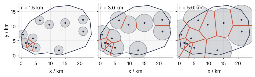
At 1.5 km only the town fires have met, and their boundaries are short straight pieces. By 3 km the town is divided up and the first boundaries run between the gauges of the open country. At 5 km most of the catchment has burnt, and the boundaries outline polygons. Each corner of a polygon is a place where three fires arrived at once.
The animation runs the fires to the end. Watch the second set of lines, the blue ones between gauges: one appears each time two fires touch for the first time, and together they cut the area into triangles. The next section is about them.

Show code
"""Growing fronts: circles grow from twelve rain gauges at one speed until they fill the plane.

Where two fronts meet, the boundary of a Voronoi cell appears; at the moment two fronts first
touch, the Delaunay edge between their gauges appears. Renders ../../assets/growing-fronts.gif.
The gauges are those of the tutorial, generated with the same seed and the same code.
Run it from any directory:

    python scene.py
"""
from pathlib import Path

import numpy as np
import matplotlib.pyplot as plt
from matplotlib.animation import FuncAnimation, PillowWriter
from matplotlib.path import Path as Outline
from scipy.spatial import Voronoi
from PIL import Image

OUT = Path(__file__).resolve().parents[2] / "assets" / "growing-fronts.gif"
INK, ACCENT, SECOND, MUTED = "#1f2a44", "#c8553d", "#2a7f9e", "#8a8f98"
plt.rcParams.update({"axes.spines.top": False, "axes.spines.right": False,
                     "axes.grid": True, "grid.alpha": 0.25, "font.size": 11})

# ---- data: the catchment and the twelve gauges of the tutorial
catchment = np.array([
    (0.5, 2.5), (4.5, 0.3), (9.0, 0.8), (13.5, 0.0), (18.0, 1.5), (22.0, 3.0), (24.0, 7.0),
    (23.5, 12.0), (21.0, 15.5), (16.5, 17.0), (11.5, 16.5), (7.0, 14.0), (3.0, 11.5), (0.0, 7.0),
])
outline = Outline(catchment)
town = np.array([4.5, 4.0])
rng = np.random.default_rng(1911)
gauges = []
while len(gauges) < 5:
    p = town + 1.2 * rng.standard_normal(2)
    if outline.contains_point(p) and all(np.hypot(*(p - q)) > 0.8 for q in gauges):
        gauges.append(p)
lo, hi = catchment.min(axis=0), catchment.max(axis=0)
while len(gauges) < 12:
    p = rng.uniform(lo, hi)
    if outline.contains_point(p) and all(np.hypot(*(p - q)) > 3.0 for q in gauges):
        gauges.append(p)
gauges = np.array(gauges)

# ---- the Voronoi edges between real gauges, closed by four ghost points far away
ghosts = (lo + hi) / 2 + 240 * np.array([(1, 0), (0, 1), (-1, 0), (0, -1)])
vor = Voronoi(np.vstack([gauges, ghosts]))
ridges = [(i, j, vor.vertices[r]) for (i, j), r in zip(vor.ridge_points, vor.ridge_vertices)
          if i < len(gauges) and j < len(gauges)]

def clip_to_disk(seg, c, r):
    """The part of segment seg within distance r of point c, or None."""
    a, d = seg[0], seg[1] - seg[0]
    qa, qb, qc = d @ d, 2 * d @ (a - c), (a - c) @ (a - c) - r * r
    disc = qb * qb - 4 * qa * qc
    if disc <= 0:
        return None
    t1 = max((-qb - np.sqrt(disc)) / (2 * qa), 0)
    t2 = min((-qb + np.sqrt(disc)) / (2 * qa), 1)
    return a + np.outer([t1, t2], seg[1] - seg[0]) if t1 < t2 else None

def touch_radius(seg, c):
    """The radius at which the front from c first reaches the edge: its distance to the segment."""
    d = seg[1] - seg[0]
    t = np.clip((c - seg[0]) @ d / (d @ d), 0, 1)
    return np.hypot(*(seg[0] + t * d - c))

touch = [touch_radius(seg, gauges[i]) for i, j, seg in ridges]

# distance to the nearest gauge on a grid over the view: the fronts are its contours
xlim, ylim = (lo[0] - 0.8, hi[0] + 0.8), (lo[1] - 0.8, hi[1] + 0.8)
xv, yv = np.meshgrid(np.linspace(*xlim, 320), np.linspace(*ylim, 240))
d_view = np.min(np.hypot(xv[..., None] - gauges[:, 0], yv[..., None] - gauges[:, 1]), axis=-1)
radii = np.concatenate([np.linspace(0.05, d_view.max() + 0.1, 96), np.full(14, d_view.max() + 0.1)])

# ---- figure, drawn once
fig, ax = plt.subplots(figsize=(7, 5.1), dpi=80, layout="constrained")
ax.plot(*np.vstack([catchment, catchment[:1]]).T, color=INK, lw=1.2)
ax.set(xlim=xlim, ylim=ylim, aspect="equal", xticks=range(0, 25, 5), yticks=range(0, 20, 5),
       xlabel="x / km", ylabel="y / km")
voronoi_lines = [ax.plot([], [], color=ACCENT, lw=1.8)[0] for _ in ridges]
delaunay_lines = [ax.plot(*gauges[[i, j]].T, color=SECOND, lw=1.2, visible=False)[0]
                  for i, j, seg in ridges]
ax.plot(*gauges.T, "o", color=INK, ms=5, zorder=3)
title = ax.set_title("", loc="left")
fronts = []

# ---- one frame: a function of the radius alone
def update(r):
    for artist in fronts:
        artist.remove()
    fronts.clear()
    fronts.append(ax.contourf(xv, yv, d_view, levels=[0, r], colors=[MUTED], alpha=0.3))
    fronts.append(ax.contour(xv, yv, d_view, levels=[r], colors=[MUTED], linewidths=1))
    for line, dline, (i, j, seg), r_touch in zip(voronoi_lines, delaunay_lines, ridges, touch):
        part = clip_to_disk(seg, gauges[i], r)
        line.set_data(*(part.T if part is not None else ([], [])))
        dline.set_visible(r >= r_touch)            # the two fronts have touched
    title.set_text(f"radius {r:.1f} km")

# ---- render, and read back what was written
OUT.parent.mkdir(exist_ok=True)
FuncAnimation(fig, update, frames=radii).save(OUT, writer=PillowWriter(fps=12))
plt.close(fig)
with Image.open(OUT) as im:
    delay = im.info["duration"]
    print(f"{OUT.name}: {im.width} x {im.height} px, {im.n_frames} frames at {delay} ms, "
          f"{im.n_frames * delay / 1000:.1f} s, {OUT.stat().st_size / 1024:,.0f} kB")
When the fires have burnt out, the territories are the Voronoi cells of the gauges, named after the mathematician Georgy Voronoi, who studied them in 1908. Hydrologists call them Thiessen polygons, after Alfred Thiessen, who used them in 1911 to average rainfall. Same polygons, two names.
To weight a gauge by its cell you need the cell's area, and there is a way to measure it that needs no geometry at all. Lay a fine grid of points over the catchment, here 0.03 km apart. Keep the points inside the outline; the standard test sends a ray from the point in any direction and counts how often it crosses the outline, and an odd count means inside. Label every remaining point with its nearest gauge and count. A gauge's area is its number of points times the area of one grid square. The weighting is then arithmetic: multiply each reading by its gauge's share of the catchment and add up the twelve products.
Show code
# distance from every grid point inside the catchment to every gauge, by broadcasting
pts = grid[inside]
dist = np.hypot(pts[:, None, 0] - gauges[:, 0], pts[:, None, 1] - gauges[:, 1])
nearest = dist.argmin(axis=1)
N = np.bincount(nearest, minlength=len(gauges))
A_grid = N * dx * dx                                      # points times the area of one grid square
share = A_grid / A_grid.sum()
print(f"grid: {len(pts):,} points inside the outline, {dx} km apart, {dx * dx * 1e6:.0f} m² each")
for p, s in sorted(zip(P, share), key=lambda ps: -ps[1])[:3]:
    print(f"  gauge reading {p:4.1f} mm: {100 * s:4.1f} % of the area")
print(f"the five town gauges: {100 * share[:5].sum():.0f} % of the area, {100 * 5 / 12:.0f} % of the votes")
grid: 343,119 points inside the outline, 0.03 km apart, 900 m² each
  gauge reading 50.1 mm: 18.5 % of the area
  gauge reading 35.3 mm: 15.8 % of the area
  gauge reading 46.1 mm: 14.5 % of the area
the five town gauges: 18 % of the area, 42 % of the votes
Of the 343,119 points inside the outline, the five town gauges get 18 % between them, against 42 % of the votes in the plain average. The 50 mm gauge in the north alone speaks for 18.5 %, as much ground as the whole town.
The other picture: link the neighbors, get triangles
Draw a line between every two gauges whose cells share an edge. These are the blue lines of the animation, and they cut the area inside the outermost gauges, the shape a rubber band stretched around all twelve would take, into triangles. That area can be cut into triangles with corners at the gauges in many ways; this one, built from the cells, is the Delaunay triangulation, after Boris Delaunay, who described it in 1934.
Show code
from scipy.spatial import Delaunay

tri = Delaunay(gauges)
vor = Voronoi(gauges)                                     # no far points: the diagram of the twelve alone

def circumcircle(a, b, c):
    """Center and radius of the circle through three points."""
    z = np.linalg.solve(2 * np.array([b - a, c - a]), [b @ b - a @ a, c @ c - a @ a])
    return z, np.hypot(*(z - a))

circles = [circumcircle(*gauges[s]) for s in tri.simplices]
centers = np.array([z for z, r in circles])
radii = np.array([r for z, r in circles])

# two circles worth showing: centered in the catchment, not too large, as far apart as possible
ok = np.flatnonzero(outline.contains_points(centers) & (radii < 6))
pairs = [(k, m) for k in ok for m in ok if k < m]
shown = max(pairs, key=lambda km: np.hypot(*(centers[km[0]] - centers[km[1]])))

def segments_cross(a, b, c, d):
    side = lambda p, q, r: np.sign((q - p)[0] * (r - p)[1] - (q - p)[1] * (r - p)[0])
    return side(a, b, c) != side(a, b, d) and side(c, d, a) != side(c, d, b)

fig, ax = plt.subplots()
draw_catchment(ax)
for i, j, seg in ridges:
    ax.plot(*seg.T, color=ACCENT, lw=1.6)
ax.triplot(*gauges.T, tri.simplices, color=SECOND, lw=1.2)
for k in shown:
    ax.add_patch(plt.Circle(centers[k], radii[k], fill=False, color=MUTED, lw=1, ls="--"))
    ax.plot(*centers[k], "o", color=MUTED, ms=4)
ax.plot(*gauges.T, "o", color=INK, ms=6, zorder=3)
plt.show()
crossing = sum(segments_cross(gauges[i], gauges[j], *seg) for i, j, seg in ridges)
print(f"{len(tri.simplices)} Delaunay triangles, {len(vor.vertices)} Voronoi cell corners")
print(f"{crossing} of {len(ridges)} Delaunay edges cross their cell edge")
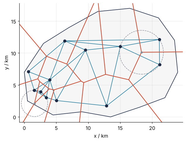
14 Delaunay triangles, 14 Voronoi cell corners
18 of 25 Delaunay edges cross their cell edge
Look at a corner where three cells meet. It is equally far from three gauges, so it is the center of a circle through all three: the circumcircle of their triangle, with the corner as its circumcenter. No gauge lies inside that circle. If one did, it would be nearer to the corner than the three, and the corner would belong to its cell instead. The two dashed circles show it for two triangles; each passes through three gauges and holds none.
Each picture is the other turned inside out. Mathematicians call such a pair dual: every piece of one stands for exactly one piece of the other, with points and areas swapped. Each gauge, a point, has a cell, an area. Each cell corner, a point, has a triangle, an area: here 14 triangles and 14 cell corners. Each cell edge has its Delaunay edge, and the two lie on lines that meet at a right angle, because the cell edge is a piece of the perpendicular bisector of the two gauges.
The segments themselves need not cross. A cell edge runs from the circumcenter of the triangle on one side of its Delaunay edge to the circumcenter of the triangle on the other side, or, along the outermost gauges, from one circumcenter outward. A circumcenter lies inside its triangle only when all three angles are below 90°. When the angle facing the Delaunay edge is over 90°, the circumcenter lies beyond that edge, on the same side as the other end of the cell edge, and the cell edge passes by without crossing. In this map 18 of the 25 pairs cross, and each of the other seven sits next to such a blunt triangle. The correspondence holds either way, so either picture can be built from the other.
Formalization
The Voronoi cell of gauge \(i\) at position \(\mathbf{p}_i\) is the set of points no farther from it than from any other gauge:
Each single condition, for one \(j\), is a half-plane: everything on gauge \(i\)'s side of the bisector of \(i\) and \(j\). A cell is the overlap of eleven half-planes, and an overlap of half-planes is always convex, a polygon without dents. A triangulation of the gauges is any way of cutting the area inside the outermost gauges into triangles whose corners are gauges and whose edges do not cross, and the same twelve points have many; the blue lines are one of them. The Delaunay triangulation is the one in which no circumcircle has a gauge inside it. The Thiessen estimate of the mean rainfall weights each reading \(P_i\) by the area \(A_i\) of its cell inside the catchment,
and the grid count of the previous section is \(A_i \approx N_i\,\Delta x\,\Delta y\), with \(N_i\) the number of grid points labeled \(i\) and \(\Delta x = \Delta y = 0.03\) km the grid spacing.
Three consequences come back every time you use either picture.
Show code
from scipy.spatial import ConvexHull

# for each triangle: distance from its circle's center to the nearest gauge not on it, over the radius
ratio = min(np.delete(np.hypot(*(gauges - z).T), s).min() / r for (z, r), s in zip(circles, tri.simplices))
n, h = len(gauges), len(ConvexHull(gauges).vertices)
edges = {tuple(sorted((s[a], s[b]))) for s in tri.simplices for a, b in [(0, 1), (1, 2), (2, 0)]}
gap = max(np.hypot(*(centers - v).T).min() for v in vor.vertices)
print(f"empty circle: smallest ratio of nearest other gauge to radius = {ratio:.2f}")
print(f"n = {n}, on the hull h = {h}")
print(f"triangles {len(tri.simplices):3d}   2n - 2 - h = {2 * n - 2 - h}")
print(f"edges     {len(edges):3d}   3n - 3 - h = {3 * n - 3 - h}")
print(f"largest distance from a cell corner to its circumcenter: {gap:.1e} km")
empty circle: smallest ratio of nearest other gauge to radius = 1.03
n = 12, on the hull h = 8
triangles  14   2n - 2 - h = 14
edges      25   3n - 3 - h = 25
largest distance from a cell corner to its circumcenter: 2.1e-14 km
The empty circle. For every triangle, take its circumcircle and the nearest gauge that is not on the triangle, and divide that gauge's distance from the center by the radius. A ratio above 1 means the circle is empty. Over the 14 triangles the smallest ratio is 1.03: one gauge sits just 3 % outside a circle. Had it sat exactly on the circle, four gauges would share one circle, and either diagonal of their quadrilateral would give a valid Delaunay triangulation. Random positions make that unlikely; gauges on a square grid make it certain.
The largest smallest angle. Wherever two triangles share an edge, their four gauges form a quadrilateral that either diagonal can split, and swapping one diagonal for the other is an edge flip, which turns one triangulation into another. Among all triangulations of a set of points, Delaunay's has the largest smallest angle. One flip shows this only locally; that it holds for the whole triangulation is a theorem, proved in the book under Further reading. Here is the flip that hurts most, found by trying every flip the map allows:
Show code
def angles(a, b, c):
    """The three angles of a triangle, in degrees."""
    out = []
    for p, q, r in [(a, b, c), (b, c, a), (c, a, b)]:
        u, v = q - p, r - p
        out.append(np.degrees(np.arccos(u @ v / (np.hypot(*u) * np.hypot(*v)))))
    return out

def cross(o, p, q):
    return (p - o)[0] * (q - o)[1] - (p - o)[1] * (q - o)[0]

flips = []
for k, s in enumerate(tri.simplices):
    for m, nb in enumerate(tri.neighbors[k]):
        if nb <= k:
            continue                                      # each interior edge once
        e1, e2 = np.delete(s, m)                          # the shared edge
        o1, o2 = s[m], (set(tri.simplices[nb]) - {e1, e2}).pop()   # the two gauges facing it
        # the flip is allowed only if the new diagonal o1-o2 crosses the old one
        if np.sign(cross(gauges[o1], gauges[o2], gauges[e1])) == np.sign(cross(gauges[o1], gauges[o2], gauges[e2])):
            continue
        before = min(angles(*gauges[[o1, e1, e2]]) + angles(*gauges[[o2, e1, e2]]))
        after = min(angles(*gauges[[e1, o1, o2]]) + angles(*gauges[[e2, o1, o2]]))
        flips.append((before - after, before, after, o1, o2, e1, e2))
_, before, after, o1, o2, e1, e2 = max(flips)

quad = [o1, e1, o2, e2]
fig, axes = plt.subplots(1, 2, figsize=(7.5, 4.2), sharex=True, sharey=True, layout="constrained")
for ax, pair, color, worst in [(axes[0], [(o1, e1, e2), (o2, e1, e2)], SECOND, before),
                               (axes[1], [(e1, o1, o2), (e2, o1, o2)], MUTED, after)]:
    for t in pair:                                        # Delaunay pair in SECOND, the flipped one in MUTED
        ax.fill(*gauges[list(t)].T, fill=False, ec=color, lw=1.6)
        z, r = circumcircle(*gauges[list(t)])
        ax.add_patch(plt.Circle(z, r, fill=False, color=MUTED, lw=1, ls="--"))
    ax.plot(*gauges[quad].T, "o", color=INK, ms=6, zorder=3)
    for t in pair:                                        # ring the gauge of the four that a circle holds
        z, r = circumcircle(*gauges[list(t)])
        swallowed = [g for g in quad if g not in t and np.hypot(*(gauges[g] - z)) < r]
        ax.plot(*gauges[swallowed].T, "o", mfc="none", mec=INK, mew=1.4, ms=15, zorder=4)
    ax.text(0.03, 0.03, f"smallest angle {worst:.0f}°", transform=ax.transAxes,
            path_effects=[withStroke(linewidth=3, foreground="white")])
    ax.set(aspect="equal", xlabel="x / km")
axes[0].set(xlim=(gauges[quad, 0].min() - 1.5, gauges[quad, 0].max() + 1.5),
            ylim=(gauges[quad, 1].min() - 2.5, gauges[quad, 1].max() + 1.5), ylabel="y / km")
plt.show()
print(f"smallest angle: Delaunay pair {before:.0f}°, flipped pair {after:.0f}°")

smallest angle: Delaunay pair 35°, flipped pair 14°
The Delaunay pair has a smallest angle of 35°, the flipped pair one of 14°, and each circle of the flipped pair swallows the gauge across the diagonal from it. Mesh generators for finite elements start from a Delaunay triangulation for this reason: thin triangles degrade the accuracy of the solution, and Delaunay's smallest angle is as large as the points allow.
Corners are circumcenters, and the counts are fixed. The cell corners from scipy.spatial.Voronoi and the circumcenters of the triangles from scipy.spatial.Delaunay come from two separate computations, and the largest distance between a corner and its circumcenter is \(2.1 \times 10^{-14}\) km: equal up to rounding in the last digits. The counts are fixed as well. With \(n\) points of which \(h\) lie on the convex hull, the rubber-band outline from above, every triangulation has \(2n - 2 - h\) triangles and \(3n - 3 - h\) edges. Here \(n = 12\) and \(h = 8\), which gives 25 edges and gives back the triangle count of the previous section. The formulas check any program's output, and they tell you how large the arrays will be before the computation runs.
See it in code
The grid count is a measurement; the exact areas come from the polygons. scipy.spatial.Voronoi computes the cells, but the outer ones are open or reach far out, because the thin triangles along the hull have circumcenters far away. Four extra points placed 240 km out, one on each side, close every real cell without changing it inside the catchment. The rule for how far: each must be farther from every point of the catchment than that point's nearest gauge, and ten times the catchment's size, as here, always is. Shapely, a library for polygons, then cuts each closed cell with the catchment outline and measures its area. Gauges given in longitude and latitude would be projected to km first, which GeoPandas from the ground up: earthquakes within 100 km of a plate boundary covers.
Show code
from shapely.geometry import Polygon

ghosts = (lo + hi) / 2 + 240 * np.array([(1, 0), (0, 1), (-1, 0), (0, -1)])   # far outside, one per side
vor_closed = Voronoi(np.vstack([gauges, ghosts]))
basin = Polygon(catchment)
cells = []
for k in range(len(gauges)):
    region = vor_closed.regions[vor_closed.point_region[k]]
    assert -1 not in region                               # every real cell is closed
    cells.append(Polygon(vor_closed.vertices[region]).intersection(basin))
A = np.array([c.area for c in cells])
thiessen = (A * P).sum() / A.sum()
tri = Delaunay(gauges)

print(f"plain average      {P.mean():5.1f} mm   ({P.mean() - true_mean:+.1f} mm)")
print(f"Thiessen average   {thiessen:5.1f} mm   ({thiessen - true_mean:+.1f} mm)")
print(f"true mean          {true_mean:5.1f} mm")
print(f"cell areas sum to {A.sum():.2f} km², the catchment is {basin.area:.2f} km²")
print(f"largest difference from the grid count: {100 * np.max(np.abs(A_grid - A) / A):.2f} %")

fig, ax = plt.subplots(figsize=(7.5, 5))
draw_catchment(ax)
norm = plt.Normalize(15, 55)
for c, p in zip(cells, P):
    ax.fill(*c.exterior.xy, color=RAIN(norm(p)), lw=0)
    ax.plot(*c.exterior.xy, color=ACCENT, lw=1.4)
for line in ax.triplot(*gauges.T, tri.simplices, color=SECOND, lw=1.2):   # white halo over the shading
    line.set_path_effects([withStroke(linewidth=3, foreground="white")])
ax.plot(*gauges.T, "o", color=INK, ms=6, zorder=3)
label_readings(ax)
ax.set_ylim(top=hi[1] + 3.2)                              # a band above the map for the three averages
ax.text(0.02, 0.98, f"plain average   {P.mean():.1f} mm\narea-weighted   {thiessen:.1f} mm\n"
        f"true mean       {true_mean:.1f} mm", transform=ax.transAxes, va="top", family="monospace")
fig.colorbar(plt.cm.ScalarMappable(norm, RAIN), ax=ax, label="rainfall / mm", shrink=0.8)
plt.show()
plain average       34.1 mm   (-6.1 mm)
Thiessen average    39.7 mm   (-0.5 mm)
true mean           40.2 mm
cell areas sum to 308.75 km², the catchment is 308.75 km²
largest difference from the grid count: 0.12 %
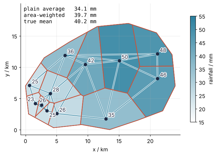
The plain average is 6.1 mm below the true mean of 40.2 mm, the Thiessen average 0.5 mm below it. The polygon areas agree with the grid counts to 0.12 % for every cell, and they add up to the catchment to the last digit printed. Thiessen is still not exact: each cell takes one reading for all of its ground, and the large cells in the north span ground that is wetter or drier than their gauge. Weights that also use how the rain varies with distance are what kriging computes, in Kriging with PyKrige: a groundwater map from forty wells and how sure it is.
Where it shows up
- Hydrology. Thiessen polygons are the classic way to turn gauge readings into areal rainfall, and catchment models offer them as a weighting option beside inverse-distance weighting and kriging. When a gauge fails, only the cells that shared an edge with it change, which is the duality at work: its Delaunay neighbors inherit its ground.
- Geology and geophysics. Terrain and horizon surfaces from scattered survey points are stored as a triangulated irregular network (TIN), Delaunay triangles with a height at each corner and a plane across each triangle. Natural neighbor interpolation, Sibson's method, weights each borehole by how much of its Voronoi cell a new point would take over.
- Materials science and solid-state physics. Grains of a metal that nucleate at random points at the same moment and grow at the same speed end up as Voronoi cells, which are the fires of the animation; the Johnson-Mehl model lets nuclei appear at different times, which bends the boundaries into hyperbolas. The Wigner-Seitz cell of a crystal, the region closer to one lattice point than to any other, is the Voronoi cell of that lattice point.
- Biology. Epithelial tissue seen from above resembles a Voronoi diagram of the cell nuclei, and vertex models of tissue mechanics are often started from one. Forest ecologists take the Voronoi cell of each tree, its "area potentially available", as a measure of how much light and water it competes for.
- Engineering. Gmsh and Shewchuk's Triangle build finite element meshes by Delaunay methods, and Triangle keeps refining until no angle falls below a bound the user sets. scikit-fem from the ground up: the sag of a membrane under pressure solves on such a mesh.
In each, the points alone decide the cells and the triangles; there is no parameter to tune, so the choice that matters is where the points go.
Further reading
scipy.spatial.Voronoiandscipy.spatial.Delaunay, both computed by the Qhull library;scipy.spatial.voronoi_plot_2ddraws a diagram in one line.- Shapely for polygons, their intersections, and their areas.
- de Berg, Cheong, van Kreveld, and Overmars, Computational Geometry: Algorithms and Applications (3rd ed., 2008), the chapters on Voronoi diagrams and Delaunay triangulations, with the proofs of the empty circle and the largest smallest angle.
- A. H. Thiessen, "Precipitation averages for large areas", Monthly Weather Review 39 (1911), where the polygons enter hydrology.
- Related tutorials on this site: Kriging with PyKrige: a groundwater map from forty wells and how sure it is, GeoPandas from the ground up: earthquakes within 100 km of a plate boundary, Finite elements: hat functions, the weak form, and a heated bar, scikit-fem from the ground up: the sag of a membrane under pressure, Vectorizing loops with NumPy: nearest neighbors of two thousand points.
- Download the notebook. It was executed with the library versions in the header.