GeoPandas from the ground up: earthquakes within 100 km of a plate boundary

The problem: how many large earthquakes strike near a plate boundary?

Plate tectonics says that large earthquakes happen where plates meet. How true is that, in numbers? The Global CMT catalog lists 5,360 earthquakes of moment magnitude Mw 6 and above from 1976 through 2020. Peter Bird's PB2002 model draws the plate boundaries as 5,819 short straight steps, 260,000 km in all, each labeled with its kind of boundary. GeoPandas, which is pandas with a column of shapes, answers the question in a handful of calls: turn the epicenters into points and the steps into lines, lay a band 100 km wide on either side of every line, and count the points inside.

The 100 km must be kilometers on the ground, not degrees on the map, because a degree of longitude shrinks toward the poles. That is the projection problem from Map projections, and getting it right is most of the work below.

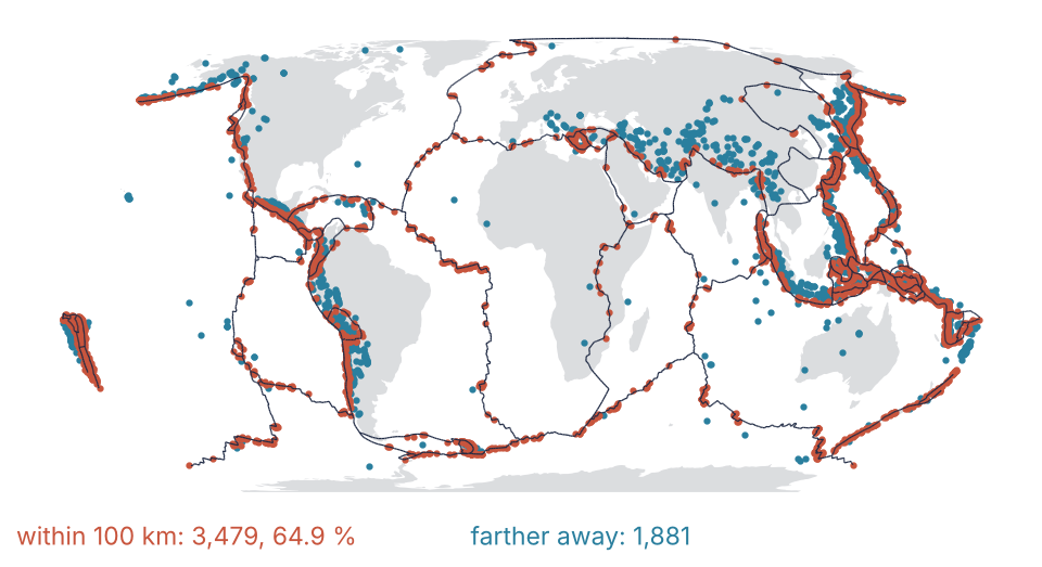
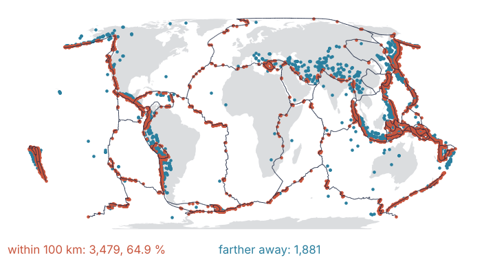
World map in the Equal Earth projection with the PB2002 plate boundaries as thin dark lines. Earthquakes of Mw 6 and above within 100 km of a boundary are red dots, those farther away blue: 64.9 % of 5,360 lie inside the band.

Of the 5,360 earthquakes, 3,479 lie within 100 km of a boundary, 64.9 %, drawn in red; the rest are blue. Step 6 draws this map; Steps 1 to 5 build the points, lines, buffers, and joins behind it.

Setup

Three files, 23.7 MB together, come from pinned addresses through pooch.retrieve, which checks each against its SHA-256 hash and reads it from its cache on every later run. The earthquakes are the Global CMT catalog through 2020, jan76_dec20.ndk, 23.0 MB (Dziewonski, Chou, and Woodhouse, J. Geophys. Res. 86, 2825, 1981; Ekström, Nettles, and Dziewonski, Phys. Earth Planet. Inter. 200-201, 1, 2012). The boundaries are Bird's PB2002_steps.dat, 0.56 MB (Bird, Geochem. Geophys. Geosyst. 4, 1027, 2003), from a copy on GitHub that matches his own file except for line endings. The land outline is Natural Earth's 1:110 million land, 0.14 MB, in the public domain. The catalog file stores each earthquake in five fixed-width lines; the last part of the cell turns it into a pandas DataFrame with one row per earthquake (year, latitude, longitude, depth) and the moment magnitude Mw computed from the scalar moment. You do not need to follow the column slicing.

import warnings
warnings.filterwarnings("ignore", message="IProgress not found")   # from tqdm, which pooch imports

import numpy as np
import pandas as pd
import geopandas as gpd
import shapely
import pyproj
import pooch
import matplotlib.pyplot as plt

plt.rcParams.update({
    "figure.figsize": (8, 4.4), "figure.dpi": 110,
    "axes.spines.top": False, "axes.spines.right": False,
    "axes.grid": True, "grid.alpha": 0.25,
    "font.size": 11, "lines.linewidth": 1.8,
})
INK, ACCENT, SECOND, MUTED = "#1f2a44", "#c8553d", "#2a7f9e", "#8a8f98"

pooch.get_logger().setLevel("WARNING")                          # no download message on the first run
ndk_path = pooch.retrieve(
    "https://www.ldeo.columbia.edu/~gcmt/projects/CMT/catalog/jan76_dec20.ndk",
    known_hash="sha256:baed5ad29a69b57344c6025b27769b1012858aa6b5c807f984696d573c0f0eb4")
steps_path = pooch.retrieve(
    "https://raw.githubusercontent.com/fraxen/tectonicplates/"
    "339b0c56563c118307b1f4542703047f5f698fae/original/PB2002_steps.dat.txt",
    known_hash="sha256:513babb111c65cd275274e2edcb249085d00e007c79d8755e1b4b79f60806f37")
land_path = pooch.retrieve(
    "https://raw.githubusercontent.com/nvkelso/natural-earth-vector/"
    "9380cca83db5f9aef52d5e762765100745f84b27/geojson/ne_110m_land.geojson",
    known_hash="sha256:9e0729ee253ca7d7a5c4ae9395fb1902264c5377c52e224d13dd85010e2835d9")

# ---- parse the catalog (not part of the lesson)
lines = open(ndk_path).read().splitlines()
hypo, expo, moment = lines[0::5], lines[3::5], lines[4::5]
catalog = pd.DataFrame({
    "year": [int(s[5:9]) for s in hypo],
    "latitude": [float(s[27:33]) for s in hypo],
    "longitude": [float(s[34:41]) for s in hypo],
    "depth": [float(s[42:47]) for s in hypo],
})
m0 = np.array([float(s[49:56]) for s in moment]) * 10.0 ** np.array([int(s[:2]) for s in expo])  # dyne cm
catalog["mw"] = 2 / 3 * (np.log10(m0) - 16.1)

print(f"{len(catalog):,} events from {catalog.year.min()} to {catalog.year.max()}, "
      f"Mw {catalog.mw.min():.1f} to {catalog.mw.max():.1f}; {(catalog.mw >= 6).sum():,} with Mw ≥ 6")

56,832 events from 1976 to 2020, Mw 4.3 to 9.1; 5,360 with Mw ≥ 6

Step 1: Turn the catalog into points with points_from_xy

A GeoDataFrame is a pandas DataFrame with one more column, geometry, that holds a shape in every row, here a point per earthquake. gpd.points_from_xy builds the points from two columns, x first, and x is longitude. The crs argument, for coordinate reference system, says what the two numbers mean. EPSG:4326 is the code for longitude and latitude in degrees on the WGS84 ellipsoid, what GPS receivers and most catalogs give.

df = catalog[catalog.mw >= 6].reset_index(drop=True)
quakes = gpd.GeoDataFrame(df, geometry=gpd.points_from_xy(df.longitude, df.latitude), crs="EPSG:4326")

print(quakes.head(3), "\n")
print("CRS:", quakes.crs.name, "  x min, y min, x max, y max:", quakes.total_bounds.round(2))

   year  latitude  longitude  depth        mw                geometry
0  1976    -28.61    -177.64   59.0  7.253639  POINT (-177.64 -28.61)
1  1976     51.60     159.33   33.0  6.131110     POINT (159.33 51.6)
2  1976    -15.76     167.87  168.0  6.307401   POINT (167.87 -15.76) 

CRS: WGS 84   x min, y min, x max, y max: [-179.99  -66.45  180.     84.95]

The geometry column prints as POINT (x y), longitude first. The last line is the check to make every time you build points: total_bounds gives the smallest and largest x and y. Here x runs from −179.99 to 180 and y from −66.45 to 84.95, the northernmost earthquake sitting on the Gakkel Ridge under the Arctic Ocean. Nothing in y goes past 90, so longitude and latitude are not swapped.

Step 2: Read the boundaries as lines and the land as polygons

The steps file is plain text, one step per line. Look at it before cleaning it:

print("".join(open(steps_path).readlines()[:2]))

   1  AF-AN   -0.438 -54.852   -0.039 -54.677  32.1  53  13.2  48    1.2   13.1  -1584   2  OTF 
   2 :AF-AN   -0.039 -54.677    0.443 -54.451  40.0  51  13.2  47    0.9   13.1  -1639   5 :OTF

Each line holds a step number, the plate pair (AF-AN, Africa and Antarctica), the longitude and latitude of both ends, the length in km, seven columns not used here, and the class, OTF for an oceanic transform fault. Bird marks a step that continues the previous one with : and a step inside an orogen with *, and the cell strips both.

shapely.linestrings takes an array of shape (n, 2, 2), n lines of two (x, y) points, and returns n LineStrings in one call, built here by stacking the two ends. The seven classes become four kinds: SUB is subduction, OCB and CCB (oceanic and continental convergent boundaries) collision, OSR and CRB (oceanic spreading ridge, continental rift) ridge, OTF and CTF transform. gpd.read_file reads the land, as it reads any GeoJSON, shapefile, or GeoPackage, CRS included.

columns = {1: "pair", 2: "lon1", 3: "lat1", 4: "lon2", 5: "lat2", 6: "length_km", 14: "cls"}
table = pd.read_csv(steps_path, sep=r"\s+", header=None, usecols=list(columns)).rename(columns=columns)
table["pair"] = table.pair.str.lstrip(":")
table["cls"] = table.cls.str.strip(":*")

kinds = {"SUB": "subduction", "OCB": "collision", "CCB": "collision", "OSR": "ridge",
         "CRB": "ridge", "OTF": "transform", "CTF": "transform"}
ends = np.stack([table[["lon1", "lat1"]].to_numpy(), table[["lon2", "lat2"]].to_numpy()], axis=1)
steps = gpd.GeoDataFrame(table.assign(kind=table.cls.map(kinds)),
                         geometry=shapely.linestrings(ends), crs="EPSG:4326")
land = gpd.read_file(land_path)

print("steps:", steps.geom_type.value_counts().to_dict(), f"  {steps.length_km.sum():,.0f} km in all, "
      f"{steps.length_km.mean():.0f} km on average, {steps.length_km.max():.0f} km at most")
print("land: ", land.geom_type.value_counts().to_dict(), "  CRS:", land.crs.to_string())
print(steps.kind.value_counts().to_string())

steps: {'LineString': 5819}   260,483 km in all, 45 km on average, 109 km at most
land:  {'Polygon': 127}   CRS: EPSG:4326
kind
ridge         2349
transform     1601
subduction    1127
collision      742

There are 5,819 LineStrings and 127 land polygons, both in EPSG:4326. At 45 km on average, a step is short enough that a straight line between its ends follows a curved boundary closely.

Step 3: Measure in kilometers with to_crs and a UTM zone

One degree of latitude is about 111 km, so 100 km is 0.9°. Buffer a point in Kamchatka by 0.9° and measure the circle with pyproj.Geod.inv, whose third output is the distance in meters on the ellipsoid:

geod = pyproj.Geod(ellps="WGS84")
circle = shapely.Point(160, 55).buffer(0.9)          # 0.9° around 160°E, 55°N
lon_min, lat_min, lon_max, lat_max = circle.bounds
_, _, north = geod.inv(160, 55, 160, lat_max)
_, _, east = geod.inv(160, 55, lon_max, 55)
print(f"the 0.9° circle reaches {north / 1000:.1f} km north and {east / 1000:.1f} km east")

the 0.9° circle reaches 100.2 km north and 57.6 km east

The circle reaches 100.2 km north but only 57.6 km east: at 55°N a degree of longitude is 0.57 of a degree of latitude. A transverse Mercator keeps distances nearly right near one meridian, and Universal Transverse Mercator, UTM, cuts the globe into 60 zones 6° wide, each with its own. get_factors returns the scale along the meridian and the parallel at a point; the cell asks for zone 54 on the equator, where a zone is widest:

utm54 = pyproj.Proj("EPSG:32654")
for lon in [141, 144, 145]:
    f = utm54.get_factors(lon, 0)
    print(f"UTM zone 54 at {lon}°E, 0°N: scale {f.meridional_scale:.4f} along the meridian, "
          f"{f.parallel_scale:.4f} along the parallel")

UTM zone 54 at 141°E, 0°N: scale 0.9996 along the meridian, 0.9996 along the parallel
UTM zone 54 at 144°E, 0°N: scale 1.0010 along the meridian, 1.0010 along the parallel
UTM zone 54 at 145°E, 0°N: scale 1.0021 along the meridian, 1.0021 along the parallel

The scale is 0.9996 at the center and 1.0010 at the zone edge, 144°E: UTM shrinks the whole zone slightly so that center and edges share the error. At 145°E, 111 km past the edge, it is 1.0021, so distances in a zone and a 100 km margin around it are off by at most 0.2 %.

The zone of a longitude is int((lon + 180) // 6) % 60 + 1, and its EPSG code is 32600 plus the zone in the north, 32700 plus the zone in the south. They differ only by 10,000 km added to y, so Step 5 uses 326xx everywhere. The cell gives the catalog a zone column and reprojects zone 54 with to_crs:

lon = 141
zone = int((lon + 180) // 6) % 60 + 1
print(f"{lon}°E is in UTM zone {zone}: EPSG:{32600 + zone} in the north, EPSG:{32700 + zone} in the south\n")

quakes["zone"] = ((quakes.longitude + 180) // 6).astype(int) % 60 + 1
quakes_z = quakes[quakes.zone == zone].to_crs(f"EPSG:{32600 + zone}")
print(quakes_z.geometry.head(3))

141°E is in UTM zone 54: EPSG:32654 in the north, EPSG:32754 in the south

23    POINT (394733.759 -5751022.169)
28     POINT (408577.68 -5717375.975)
44     POINT (399059.565 -508513.459)
Name: geometry, dtype: geometry

x and y are now in meters. The first two rows lie at 52°S, south of Australia, where the northern code makes y negative, −5,751 km.

Step 4: Buffer the boundaries and join the earthquakes in one zone

Zone 54 runs from 138°E to 144°E, pole to pole: Japan and the Izu-Bonin arc in the north, the ridge between Australia and Antarctica in the south. The cell projects only the boundary steps near the zone, because those on the far side of the globe come out distorted, and buffers each by 100,000 m. A buffer is the polygon of all points within that distance of a shape, here a band with rounded ends.

Near means within 20° of longitude of the zone's central meridian, for a reason Step 5 gives. Zone 1 is centered on 177°W and each zone lies 6° east of the last, so zone n is centered on 6n − 183 degrees, 141°E here. A plain difference fails across 180°: 179°W minus 141°E is −320°, 40° east the short way. Add 180, take the remainder by 360, which Python keeps between 0 and 360 even for a negative number, and subtract 180: every difference lands between −180° and 180°, east positive.

A join pairs the rows of two tables. In pandas the pairing key is a shared column; in a spatial join it is a geometric relation, here "the point lies within the polygon", so every earthquake is paired with every buffer that contains it.

lon0 = 6 * zone - 183                                   # central meridian of the zone, 141°E
offset = (steps.lon1 - lon0 + 180) % 360 - 180          # degrees east of it, -180 to 180
near = steps[offset.abs() < 20].to_crs(quakes_z.crs)
buffers = gpd.GeoDataFrame(near[["pair", "kind"]], geometry=near.buffer(100_000), crs=near.crs)

joined = gpd.sjoin(quakes_z, buffers, predicate="within").sort_index()
print(joined[["year", "mw", "depth", "index_right", "pair", "kind"]].head(6).round(1), "\n")
print(f"zone {zone}: {len(quakes_z)} earthquakes, {len(joined.index.unique())} of them within 100 km "
      f"of a boundary, {len(joined):,} rows in the join")

    year   mw  depth  index_right   pair       kind
23  1976  6.0   33.0         1016  AU-AN  transform
23  1976  6.0   33.0         1017  AU-AN  transform
23  1976  6.0   33.0         1018  AU-AN      ridge
23  1976  6.0   33.0         1019  AU-AN  transform
23  1976  6.0   33.0         1020  AU-AN  transform
28  1976  6.3   33.0         1016  AU-AN  transform 

zone 54: 353 earthquakes, 187 of them within 100 km of a boundary, 1,000 rows in the join

The join has one row per pair of earthquake and buffer, so an earthquake near several steps appears several times: earthquake 23 lies within five buffers of the Australia-Antarctica boundary, and index_right is each step's row in steps. index.unique() counts the distinct earthquakes in the 1,000 rows: 187 of the 353 in the zone.

Step 5: Repeat it for every zone

Every zone needs its own CRS, so the Step 4 code goes into a loop over quakes.groupby("zone"). A transverse Mercator breaks down 90° from its central meridian, so the 20° window of Step 4 keeps the far side out.

The window must hold every step that could pass within 100 km of an earthquake in the zone, and the cell selects a step by its first end alone. Add up how far that end can lie from the central meridian: 3° for an earthquake at the zone edge, about 10° for 100 km of longitude at 85°N, where the northernmost earthquake is, and the step's whole width, because the first end may be the far one. The last line of the cell measures that width, at most 4.1° poleward of 75°, so the sum is 3° + 10° + 4.1° = 17°, inside 20°. Steps that far out are distorted beyond the 0.2 % of Step 3, but too far from the zone's earthquakes to change a count.

The loop also runs a second join for Step 6: gpd.sjoin_nearest pairs each earthquake with its nearest step up to max_distance and writes the distance into distance_m, so an earthquake near steps of two kinds counts once. Steps that share an end can tie and give two rows; the cell keeps one. Each zone's result drops its geometry before pd.concat, because GeoPandas refuses to stack geometries in different CRSs.

inside_parts, nearest_parts = [], []
for zone, group in quakes.groupby("zone"):
    crs = f"EPSG:{32600 + zone}"
    offset = (steps.lon1 - (6 * zone - 183) + 180) % 360 - 180
    near = steps[offset.abs() < 20].to_crs(crs)
    buffers = gpd.GeoDataFrame(near[["kind"]], geometry=near.buffer(100_000), crs=crs)
    group = group.to_crs(crs)
    inside_parts.append(gpd.sjoin(group, buffers, predicate="within").drop(columns="geometry"))
    nearest = gpd.sjoin_nearest(group, near[["kind", "geometry"]], max_distance=100_000,
                                distance_col="distance_m")
    nearest_parts.append(nearest[~nearest.index.duplicated()].drop(columns="geometry"))  # ties: keep one

inside = pd.concat(inside_parts)
nearest = pd.concat(nearest_parts).sort_index()
n_in = len(inside.index.unique())
print(f"{n_in:,} of {len(quakes):,} earthquakes, {100 * n_in / len(quakes):.1f} %, "
      "lie within 100 km of a plate boundary")
print("sjoin_nearest finds the same ones:", set(nearest.index) == set(inside.index))

span = ((steps.lon2 - steps.lon1 + 180) % 360 - 180).abs()   # degrees of longitude per step
polar = steps[["lat1", "lat2"]].abs().max(axis=1) >= 75
print(f"widest step in longitude: {span[polar].max():.1f}° poleward of 75°, {span[~polar].max():.1f}° elsewhere")

3,479 of 5,360 earthquakes, 64.9 %, lie within 100 km of a plate boundary
sjoin_nearest finds the same ones: True
widest step in longitude: 4.1° poleward of 75°, 1.7° elsewhere

3,479 of 5,360, 64.9 %, the number on the map. The nearest join finds exactly the same earthquakes, so buffers and distances agree in all 60 zones.

Step 6: Group by boundary type and draw the map

groupby("kind") on the nearest-join table counts the earthquakes inside by the kind of their nearest step, and dividing by each kind's boundary length turns counts into a rate. Depth gets a crosstab of three bands against inside and outside. The bins start at minus infinity because eight earthquakes have a depth of 0 km, and pd.cut leaves out the left edge of a bin.

count = nearest.groupby("kind").size().sort_values(ascending=False)
km = steps.groupby("kind").length_km.sum()
for kind, n in count.items():
    print(f"{kind:10s} {n:5,d}   {100 * n / count.sum():3.0f} % of those inside   "
          f"{1000 * n / km[kind]:5.1f} per 1,000 km of boundary")

quakes["inside"] = quakes.index.isin(inside.index)
band = pd.cut(quakes.depth, [-np.inf, 70, 300, np.inf], labels=["≤ 70 km", "70 to 300 km", "> 300 km"])
depth = pd.crosstab(band, quakes.inside).rename(columns={True: "inside", False: "outside"})
depth["share inside / %"] = (100 * depth.inside / (depth.inside + depth.outside)).round().astype(int)
print()
print(depth[["inside", "outside", "share inside / %"]].rename_axis(index="depth", columns=None))

subduction 1,566    45 % of those inside    30.5 per 1,000 km of boundary
transform    895    26 % of those inside    12.1 per 1,000 km of boundary
ridge        547    16 % of those inside     5.8 per 1,000 km of boundary
collision    471    14 % of those inside    11.6 per 1,000 km of boundary

              inside  outside  share inside / %
depth                                          
≤ 70 km         3014     1123                73
70 to 300 km     370      447                45
> 300 km          95      311                23

Subduction zones take 45 % of the earthquakes inside, and per 1,000 km of boundary five times as many as ridges, 30.5 against 5.8. The deeper an earthquake, the less likely it lies within 100 km of a boundary in map view: 73 % of the shallow ones do, 23 % of those below 300 km, which lie in slabs dipping away from the trench. The outside third is still mostly shallow, 1,123 of 1,881, because shallow earthquakes outnumber the intermediate band five to one, 4,137 against 817.

The map reprojects every layer into Equal Earth, EPSG:8857, and draws each with its own .plot, the earthquakes inside last so they sit on top.

across = (steps.lon1 - steps.lon2).abs() > 180          # six steps jump across 180°, see Pitfalls
world = quakes.to_crs("EPSG:8857")                      # Equal Earth

fig, ax = plt.subplots()
land.to_crs(world.crs).plot(ax=ax, color=MUTED, alpha=0.3, lw=0)
steps[~across].to_crs(world.crs).plot(ax=ax, color=INK, lw=0.6)
world[~world.inside].plot(ax=ax, color=SECOND, markersize=4)
world[world.inside].plot(ax=ax, color=ACCENT, markersize=4)
ax.set_axis_off()
ax.text(0.0, -0.06, f"within 100 km: {n_in:,}, {100 * n_in / len(quakes):.1f} %", color=ACCENT,
        transform=ax.transAxes)
ax.text(0.45, -0.06, f"farther away: {len(quakes) - n_in:,}", color=SECOND, transform=ax.transAxes)
plt.show()

World map in the Equal Earth projection with the PB2002 plate boundaries as thin dark lines. Earthquakes of Mw 6 and above within 100 km of a boundary are red dots, those farther away blue: 64.9 % of 5,360 lie inside the band.

Pitfalls

Buffering in degrees. Buffer the unprojected steps by 0.9° and GeoPandas warns once and goes ahead:

with warnings.catch_warnings(record=True) as caught:
    warnings.simplefilter("always")
    degree_buffers = gpd.GeoDataFrame(geometry=steps.buffer(0.9), crs=steps.crs)
print(str(caught[0].message).split(".")[0] + ".")

inside_deg = quakes.index.isin(gpd.sjoin(quakes, degree_buffers, predicate="within").index)
print(f"inside by the degree buffer: {100 * inside_deg.mean():.1f} %, against {100 * quakes.inside.mean():.1f} %; "
      f"{(inside_deg & ~quakes.inside).sum()} counted in that are not, {(~inside_deg & quakes.inside).sum()} missed")

Geometry is in a geographic CRS.
inside by the degree buffer: 64.3 %, against 64.9 %; 112 counted in that are not, 146 missed

A share of 64.3 % against 64.9 % looks like rounding, but 258 earthquakes are on the wrong side: 112 counted in that are not, 146 missed. Part of the cause is Step 3, where a degree of longitude shrinks toward the poles; the rest is the next pitfall. The fix is to_crs into a projected CRS that is accurate where you measure, before any buffer or distance.

Lines across the antimeridian. Six PB2002 steps run from just west of 180° to just east of it, from the Pacific-Antarctic ridge to the Aleutians. Their ends differ by almost 360° in longitude, and a straight line between them goes the long way round:

crossing = steps[across]
from_crossing = quakes.index.isin(gpd.sjoin(quakes, degree_buffers[across], predicate="within").index)
print(pd.DataFrame({
    "pair": crossing.pair, "latitude": crossing.lat1.round(1), "file / km": crossing.length_km,
    "Equal Earth / km": (crossing.to_crs("EPSG:8857").length / 1000).round().astype(int),
    "UTM zone 1 / km": (crossing.to_crs("EPSG:32601").length / 1000).round().astype(int),
}).to_string(index=False))
print(f"false positives of the degree buffer near these six: {(from_crossing & ~quakes.inside).sum()}")

 pair  latitude  file / km  Equal Earth / km  UTM zone 1 / km
PA-AN     -65.7       47.1             24424               47
KE/PA     -37.5       82.1             31089               82
KE-AU     -31.8       71.3             31942               71
NA/PA      50.5       78.5             28274               79
BR-AU     -15.7       41.6             33850               42
PA-BR     -15.2       62.1             33857               62
false positives of the degree buffer near these six: 112

On the Equal Earth map each is 24,000 to 34,000 km long, a line across the world, and buffered in degrees it becomes a band around the globe; all 112 false positives of the degree buffer lie in those bands. In UTM zone 1, centered on 177°W, they are 42 to 82 km long, as the file says. Find such lines with (lon1 - lon2).abs() > 180, measure them in a projected CRS centered near them, and for a world map drop them, as Step 6 does, or split them at 180°.

Longitude and latitude swapped. The catalog file, like most catalogs, gives latitude before longitude, and points_from_xy(df.latitude, df.longitude) raises nothing. The symptom is earthquakes in the wrong ocean, or a total_bounds with y beyond ±90, here up to 180. The fix is a habit: x is longitude, and total_bounds is the first thing you print after building points.

Variations

Volcanoes instead of earthquakes. Turn a list of Holocene volcanoes into points with points_from_xy; the zone loop and both joins stay as they are.
Depth against distance from a subduction zone. Run sjoin_nearest against the SUB steps only and plot depth against distance_m, which shows the dipping band of earthquakes in the sinking plate, the Wadati-Benioff zone.
Read a shapefile. gpd.read_file opens Natural Earth's zipped shapefile, ne_110m_land.zip, with the same call as the GeoJSON.
Distance as a variable, not a threshold. Leave out max_distance and draw a histogram of distance_m; the 100 km then becomes a choice you can see.

Cheat sheet

gdf = gpd.GeoDataFrame(df, geometry=gpd.points_from_xy(df.lon, df.lat), crs="EPSG:4326")  # x is longitude
gdf.total_bounds                                     # x min, y min, x max, y max: check |y| <= 90
land = gpd.read_file("land.geojson")                 # GeoJSON, shapefile, GeoPackage; CRS comes along
zone = int((lon + 180) // 6) % 60 + 1                # UTM zone of a longitude
epsg = 32600 + zone                                  # north; 32700 + zone south, same distances
local = gdf.to_crs(f"EPSG:{epsg}")                   # x and y in meters
bands = local.buffer(100_000)                        # 100 km, only in a projected CRS
hits = gpd.sjoin(points, polygons, predicate="within")   # one row per (point, polygon) pair
hits.index.unique()                                  # each point once
gpd.sjoin_nearest(points, lines, max_distance=1e5, distance_col="distance_m")  # nearest line and its distance