The wave equation: why a string plucked at a fifth has no fifth harmonic

The question

The A string of a classical guitar is 65 cm long and sounds at 110 Hz. Pluck it 13 cm from the bridge, a fifth of its length, and record its displacement with a pickup 3 cm from the bridge, 44,100 samples a second for one second. The record below is not measured: it is computed from the exact solution of the wave equation for this string, so that the answer can be checked later. Here are its first 20 ms and its spectrum, how much of each frequency it contains.

Show code

Copy

import numpy as np
import matplotlib.pyplot as plt

plt.rcParams.update({
    "figure.figsize": (7, 4.4), "figure.dpi": 110,
    "axes.spines.top": False, "axes.spines.right": False,
    "axes.grid": True, "grid.alpha": 0.25,
    "font.size": 11, "lines.linewidth": 1.8,
})
INK, ACCENT, SECOND, MUTED = "#1f2a44", "#c8553d", "#2a7f9e", "#8a8f98"

# The record is computed from the exact solution of the sections below, so that the
# answer can be checked at the end. Pretend you have not seen this cell.
L, F1 = 0.65, 110.0        # the A string: length / m, fundamental / Hz
C = 2 * L * F1             # wave speed / (m/s)
BETA = 0.2                 # pluck point, as a fraction of L from the bridge
X_PICK = 0.03              # pickup position / m from the bridge
FS = 44100                 # samples per second

def F(s):
    """The pluck, height 1 at BETA*L, continued beyond both ends as its upside-down mirror image."""
    return np.interp(np.mod(s, 2 * L), [0, BETA * L, L, 2 * L - BETA * L, 2 * L], [0, 1, 0, -1, 0])

def u(x, t):
    """Displacement of the string, in units of the pluck height h."""
    return 0.5 * (F(x - C * t) + F(x + C * t))

t = np.arange(FS) / FS
record = u(X_PICK, t)
freq = np.fft.rfftfreq(t.size, d=1 / FS)
amp = 2 * np.abs(np.fft.rfft(record)) / t.size
level = 20 * np.log10(np.maximum(amp, 1e-12) / amp[110])     # dB relative to the fundamental

fig, (ax1, ax2) = plt.subplots(2, 1, layout="constrained")
first = t < 0.020
ax1.plot(1e3 * t[first], record[first], color=INK)
t_up = 1e3 * t[np.flatnonzero(np.diff(np.sign(record - 0.1)) > 0)[0]]   # a rising edge / ms
T_ms = 1e3 * 2 * L / C
ax1.annotate("", (t_up + T_ms, 0.29), (t_up, 0.29), arrowprops=dict(arrowstyle="<->", color=MUTED, lw=1))
ax1.text(t_up + T_ms / 2, 0.30, f"{T_ms:.2f} ms", color=MUTED, ha="center", va="bottom")
ax1.set(xlabel="t / ms", ylabel="u / h", xlim=(0, 20), ylim=(-0.09, 0.4))
ax2.plot(freq, level, color=INK, lw=1.2)
ax2.annotate("110", (110, 0), xytext=(0, 4), textcoords="offset points", ha="center")
ax2.vlines([550, 1100, 1650, 2200], -60, -6, color=MUTED, lw=1, ls="--")
ax2.text(560, 4, "nothing at 550 Hz and its multiples", color=MUTED, va="bottom")
ax2.set(xlabel="f / Hz", ylabel="level / dB", xlim=(0, 2500), ylim=(-60, 16),
        xticks=[0, 550, 1100, 1650, 2200])
plt.show()
print(f"wave speed c = 2 L f1 = {C:.0f} m/s, period 2L/c = {1e3 * 2 * L / C:.2f} ms")

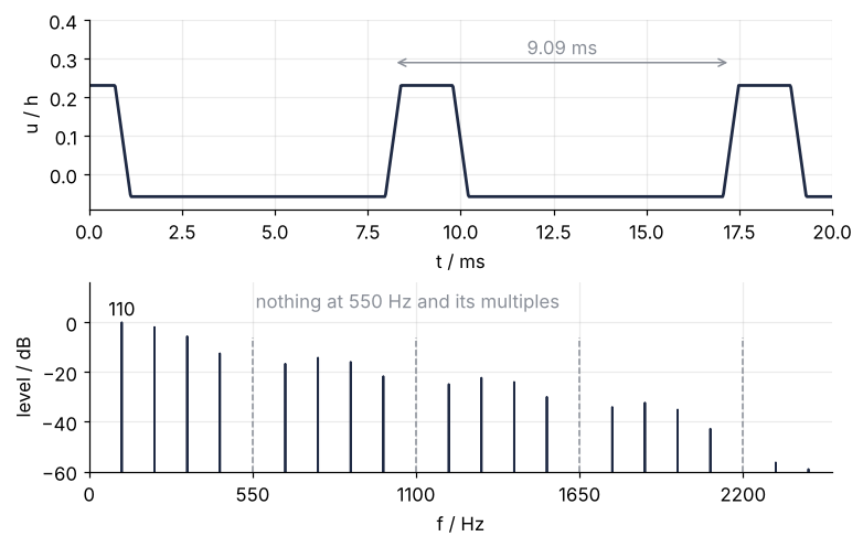
wave speed c = 2 L f1 = 143 m/s, period 2L/c = 9.09 ms

Two things are obvious. The signal repeats every 9.09 ms, and the spectrum has peaks at 110, 220, 330, and 440 Hz: a note and its overtones at whole multiples, the harmonics every guitarist knows. How tall each peak stands depends on the string and also on where the pickup sits, and the sections below take those two apart.

Less obvious: 550 Hz is missing. So are 1,100, 1,650, and 2,200 Hz, every fifth harmonic, while the sixth to the ninth come back. The finger pulled at a fifth of the length and every fifth harmonic is gone, which is hard to take for a coincidence. The question this tutorial answers is what the string's equation says about which frequencies a string can make at all, and how much of each a given pluck puts in. The wave equation answers it twice, once as two waves running along the string and once as shapes that swing in place.

The idea: the pluck splits into two halves that run apart

Pull the string into a triangle and hold it there. That triangle is two triangles of half the height, stacked on top of each other. Let go, and one of them runs toward the nut and the other toward the bridge, both at the same speed and both keeping their shape exactly. For this string the speed is 143 m/s, set by its tension and its mass.

An end of the string cannot move. Picture, beyond the end, an upside-down mirror image of the arriving half, coming in from outside at the same speed: at the end point the two cancel at every instant, and as the real half runs off the string, the image runs on. So a half comes back from an end upside down. Here is the string at three moments, with both halves continued past the ends, faint where they are only images:

Show code

Copy

x_wide = np.linspace(-0.30, 0.95, 1251)
on = (x_wide >= 0) & (x_wide <= L)

def draw_halves(ax, t):
    """The string at time t, with its two traveling halves, faint where they lie beyond the ends."""
    halves = [(0.5 * F(x_wide - C * t), ACCENT), (0.5 * F(x_wide + C * t), SECOND)]
    for half, color in halves:
        ax.plot(100 * x_wide, np.where(on, np.nan, half), color=color, lw=1.2, alpha=0.35)
        ax.plot(100 * x_wide[on], half[on], color=color, lw=1.4)
    ax.plot(100 * x_wide[on], u(x_wide[on], t), color=INK, lw=2.6)
    for end in [0, 100 * L]:
        ax.axvline(end, color=MUTED, lw=1.2)
    ax.set(ylim=(-1.1, 1.15), ylabel="u / h")

fig, axes = plt.subplots(3, 1, figsize=(7, 6.2), sharex=True, layout="constrained")
for ax, t_ms in zip(axes, [0.0, 0.5, 1.5]):
    draw_halves(ax, 1e-3 * t_ms)
    ax.text(0.99, 0.9, f"t = {t_ms} ms", transform=ax.transAxes, ha="right", va="top")
axes[0].plot(100 * BETA * L, 1, "o", color=MUTED, ms=6)
axes[0].text(22, 0.2, "both halves", color=MUTED, va="top")
axes[0].text(1, -0.9, "bridge", color=MUTED)
axes[0].text(100 * L + 1, -0.9, "nut", color=MUTED)
axes[-1].set(xlabel="x / cm from the bridge", xlim=(-30, 95))
plt.show()

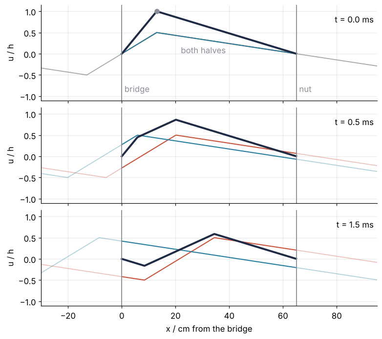
At 0.5 ms the single corner has become two, joined by a straight stretch of string that sits lower than the corner did. At 1.5 ms the corner that ran toward the bridge has gone past it, and what is on the string near the bridge is the image's corner, upside down and coming back. Over one full period it looks like this:

"""Traveling halves: a plucked string as two half-height copies of the pluck running apart.

Renders ../../assets/traveling-halves.gif, one period of the A string of a guitar plucked
at a fifth of its length. Run it from any directory:

    python scene.py
"""
from pathlib import Path

import numpy as np
import matplotlib.pyplot as plt
from matplotlib.animation import FuncAnimation, PillowWriter
from PIL import Image

OUT = Path(__file__).resolve().parents[2] / "assets" / "traveling-halves.gif"
INK, ACCENT, SECOND, MUTED = "#1f2a44", "#c8553d", "#2a7f9e", "#8a8f98"
plt.rcParams.update({"axes.spines.top": False, "axes.spines.right": False,
                     "axes.grid": True, "grid.alpha": 0.25, "font.size": 11})

# ---- the string: length / m, fundamental / Hz, pluck point as a fraction of L from the bridge
L, F1, BETA = 0.65, 110.0, 0.2
C = 2 * L * F1


def F(s):
    """The pluck, height 1, continued beyond both ends as its upside-down mirror image."""
    return np.interp(np.mod(s, 2 * L), [0, BETA * L, L, 2 * L - BETA * L, 2 * L], [0, 1, 0, -1, 0])


x = np.linspace(-0.30, 0.95, 1251)
on = (x >= 0) & (x <= L)
frames = np.linspace(0, 1 / F1, 108, endpoint=False)      # one period; the loop closes without a repeated frame

# ---- figure, drawn once
fig, ax = plt.subplots(figsize=(7, 3.0), dpi=80, layout="constrained")
ax.axvspan(-30, 0, color=MUTED, alpha=0.08, lw=0)
ax.axvspan(100 * L, 95, color=MUTED, alpha=0.08, lw=0)
for end, name in [(0, "bridge"), (100 * L, "nut")]:
    ax.axvline(end, color=MUTED, lw=1.2)
    ax.text(end + 1, -1.0, name, color=MUTED)
ax.axhline(0, color=MUTED, lw=1, ls="--")
right_faint, = ax.plot([], [], color=ACCENT, lw=1.4, alpha=0.35)
left_faint, = ax.plot([], [], color=SECOND, lw=1.4, alpha=0.35)
right, = ax.plot([], [], color=ACCENT, lw=1.6, label="running to the nut")
left, = ax.plot([], [], color=SECOND, lw=1.6, label="running to the bridge")
string, = ax.plot([], [], color=INK, lw=3, label="string")
clock = ax.text(0.99, 0.96, "", transform=ax.transAxes, ha="right", va="top")
ax.set(xlim=(-30, 95), ylim=(-1.15, 1.15), xlabel="x / cm from the bridge", ylabel="u / h")
ax.legend(frameon=False, loc="lower left", bbox_to_anchor=(0, 1), ncol=3, borderaxespad=0.2)


# ---- one frame: a function of the time alone
def update(t):
    half_r, half_l = 0.5 * F(x - C * t), 0.5 * F(x + C * t)
    right_faint.set_data(100 * x, np.where(on, np.nan, half_r))
    left_faint.set_data(100 * x, np.where(on, np.nan, half_l))
    right.set_data(100 * x[on], half_r[on])
    left.set_data(100 * x[on], half_l[on])
    string.set_data(100 * x[on], (half_r + half_l)[on])
    clock.set_text(f"t = {1e3 * t:4.2f} ms")


# ---- render, and read back what was written
OUT.parent.mkdir(exist_ok=True)
FuncAnimation(fig, update, frames=frames).save(OUT, writer=PillowWriter(fps=12))
plt.close(fig)
with Image.open(OUT) as im:
    print(f"{OUT.name}: {im.width} x {im.height} px, {im.n_frames} frames, "
          f"{OUT.stat().st_size / 1024:,.0f} kB")

The cell below checks what the pictures claim. It finds the corners as the points where the string bends most sharply, so that you can see each one move by \(ct\), and it measures how far the string is from its starting shape after one round trip:

x = np.linspace(0, L, 6501)                        # 0.1 mm apart

def corners(t):
    """Positions / cm where the string bends: the largest second differences."""
    bend = np.abs(np.diff(u(x, t), 2))
    return np.unique(np.round(100 * x[1:-1][bend > 0.5 * bend.max()], 1))

for t_ms in [0.0, 0.5, 1.5]:
    found = "  ".join(f"{p:5.1f}" for p in corners(1e-3 * t_ms))
    print(f"t = {t_ms:3.1f} ms   c t = {100 * C * t_ms * 1e-3:4.1f} cm   corners at {found} cm")

period = 2 * L / C
print(f"the corner running to the bridge arrives after {1e3 * BETA * L / C:.2f} ms")
print(f"after one period, {1e3 * period:.2f} ms, the string differs from its start by "
      f"{np.abs(u(x, period) - u(x, 0)).max():.0e} h")

t = 0.0 ms   c t =  0.0 cm   corners at  13.0 cm
t = 0.5 ms   c t =  7.2 cm   corners at   5.9   20.2 cm
t = 1.5 ms   c t = 21.4 cm   corners at   8.5   34.4 cm
the corner running to the bridge arrives after 0.91 ms
after one period, 9.09 ms, the string differs from its start by 9e-16 h

At 0.5 ms the corners sit 7.2 cm either side of 13 cm, which is \(ct\). At 1.5 ms one is at 34.4 cm, 21.4 cm out, and the other at 8.5 cm: 13 cm to the bridge and the rest of the 21.4 cm back. The corner reached the bridge after 0.91 ms. After 9.09 ms the string differs from its start by 9e-16 h, zero to rounding.

None of this depends on the triangle. Any shape splits into two halves, and after each has gone a full \(2L\) and been flipped twice, the string is where it started, so every motion of this string repeats after \(2L/c\). A signal that repeats every \(T\) contains only whole multiples of \(1/T\), and so the string can sound 110, 220, 330 Hz and nothing in between. Which of those multiples a pluck actually puts in, the running halves do not tell you.

The same motion as a sum of standing waves

The same string can be described with shapes that do not travel but swing in place: the sine arches \(\sin(n\pi x/L)\), pinned at both ends, with one hump for \(n = 1\), two for \(n = 2\), and so on. Arch \(n\) is a wave of length \(2L/n\), and at 143 m/s that swings \(n\) times as fast as the first, at \(n \cdot 110\) Hz. These are the string's modes. The harmonics are their frequencies.

What a weight is. Any starting shape that is pinned at both ends is a sum of these arches, each with a weight \(b_n\) that says how much of mode \(n\) is in the shape. You find it with the same probe as in the Fourier transform: multiply the shape by arch \(n\) point by point and take twice the average over the string. For a shape made of straight pieces, the straight stretches average out against the arch and only the corners leave something behind, in proportion to the arch's height at the corner (Formalization shows why). A mode with a node at the corner gets no weight at all.

x = np.linspace(0, L, 2001)

def weights(shape, n_max=20):
    """b_n / h for n = 1 to n_max: twice the average of shape times arch n."""
    n = np.arange(1, n_max + 1)[:, None]
    return 2 / L * np.trapezoid(shape * np.sin(n * np.pi * x / L), x, axis=1)

b = weights(u(x, 0))
for n, bn in enumerate(b[:6], start=1):
    print(f"b_{n} = {bn:.4g} h")

b_1 = 0.7444 h
b_2 = 0.3011 h
b_3 = 0.1338 h
b_4 = 0.04653 h
b_5 = -1.868e-17 h
b_6 = -0.02068 h

Mode 5 has a node at 13 cm, exactly where the finger pulled, and its weight prints as -2e-17 h, which is rounding: the pluck never sets it going. Here are the first weighted modes, and the sums of the first 1, 4, and 20 against the triangle at release. The cell then lets each sum swing through a full period and prints its largest difference from the traveling halves of the previous section, which Formalization calls d'Alembert's solution:

Show code

Copy

def mode_sum(x, t, weights_n):
    n = np.arange(1, weights_n.size + 1)[:, None]
    return (weights_n[:, None] * np.sin(n * np.pi * x / L) * np.cos(2 * np.pi * n * F1 * t)).sum(axis=0)

fig, (ax1, ax2) = plt.subplots(2, 1, figsize=(7, 5.2), sharex=True, layout="constrained")
# each label sits at a hump of its mode where no other mode crosses: (hump x / cm, above or below)
for n, x_hump, side in [(1, 32.5, 1), (2, 16.25, 1), (3, 32.5, -1), (4, 40.6, 1), (6, 5.4, -1)]:
    mode = b[n - 1] * np.sin(n * np.pi * x / L)
    ax1.plot(100 * x, mode, color=MUTED, lw=1.1)
    y_hump = b[n - 1] * np.sin(n * np.pi * x_hump / 100 / L)
    ax1.annotate(f"n = {n}", (x_hump, y_hump), xytext=(0, 3 * side), textcoords="offset points",
                 ha="center", va="bottom" if side > 0 else "top")
ax1.plot(100 * x, 0.08 * np.sin(5 * np.pi * x / L), color=MUTED, lw=1.1, ls="--")
ax1.plot(100 * BETA * L, 0, "o", color=INK, ms=6)
ax1.text(100 * BETA * L + 1, -0.12, "n = 5: weight 0", va="top")
ax1.set(ylabel="b_n sin(nπx/L) / h", ylim=(-0.3, 0.88))
ax2.plot(100 * x, u(x, 0), color=INK, lw=2.4)
# the sums are made of the gray modes above, so they are gray too, darker with more modes
for n_modes, alpha, (x_label, y_label, ha) in [(1, 0.45, (40, 0.62, "left")), (4, 0.75, (24, 0.98, "left")),
                                               (20, 1.0, (12.5, 1.02, "right"))]:
    ax2.plot(100 * x, mode_sum(x, 0, b[:n_modes]), color=MUTED, alpha=alpha, lw=1.4)
    ax2.text(x_label, y_label, f"{n_modes} mode" + "s" * (n_modes > 1), color=MUTED, ha=ha)
ax2.set(xlabel="x / cm from the bridge", ylabel="u / h", xlim=(0, 100 * L), ylim=(-0.05, 1.15))
plt.show()

x_check = np.linspace(0, L, 400)
instants = np.linspace(0, period, 60, endpoint=False)
for n_modes in [5, 20, 50]:
    w = weights(u(x, 0), n_modes)
    worst = max(np.abs(mode_sum(x_check, t, w) - u(x_check, t)).max() for t in instants)
    print(f"{n_modes:2d} modes: largest difference from d'Alembert over one period {100 * worst:4.1f} % of h")

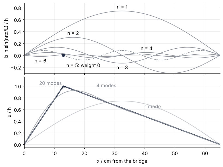
 5 modes: largest difference from d'Alembert over one period 12.0 % of h
20 modes: largest difference from d'Alembert over one period  3.0 % of h
50 modes: largest difference from d'Alembert over one period  1.1 % of h

One mode is a smooth hump, four already lean toward the corner, and twenty stay within 3.0 % of h of the traveling halves at every instant of a period, the error sitting at the corners, which smooth arches can only round off. Five modes miss by 12.0 %, fifty by 1.1 %. Two views of one string, then: the running halves say the motion repeats every 9.09 ms, the weights say how much of each multiple of 110 Hz it carries.

Any shape, numerically. The average does not need a formula for the shape. Pull the string with two fingers to the same height at 13 cm and at 52 cm, so that it is flat between them, and predict before computing. The shape is symmetric about the middle of the string, and every even arch is antisymmetric about it, so the even weights cancel. The two corners sit at 1/5 and 4/5 of the length, and both are nodes of every fifth arch, so those weights vanish too.

two_fingers = np.interp(x, [0, 0.13, 0.52, L], [0, 1, 1, 0])
b_two = weights(two_fingers)
present = np.flatnonzero(np.abs(b_two) > 1e-6) + 1
print("harmonics present among the first 20:", *present)
print(f"b_1 = {b_two[0]:.3f} h,  b_3 = {b_two[2]:.3f} h")

harmonics present among the first 20: 1 3 7 9 11 13 17 19
b_1 = 1.191 h,  b_3 = 0.214 h

The survivors are 1, 3, 7, 9, 11, 13, 17, and 19, as predicted. The fundamental is stronger than the triangle's, 1.191 h against 0.744 h, because more of the string was pulled aside.

Formalization

Take a short piece of string with tension \(\tau\) and mass per length \(\mu\). The tension pulls along the string at both ends of the piece. If the string is straight, the pulls cancel; if it is curved, they point in slightly different directions and leave a sideways force proportional to the curvature, \(\partial^2 u/\partial x^2\) for small slopes. Newton's second law for the piece is the wave equation:

Here \(u(x, t)\) is the sideways displacement. The ends are fixed, \(u(0, t) = u(L, t) = 0\), and a plucked string starts from rest, \(\partial u/\partial t = 0\) at \(t = 0\), in the shape of the pluck.

Any function of \(x - ct\) solves this equation, and so does any function of \(x + ct\): differentiate either twice and both sides give \(c^2\) times its second derivative. The general solution is a shape moving right plus a shape moving left, \(u = f(x - ct) + g(x + ct)\). Released from rest, the two are equal halves of the start,

where \(F\) is the pluck on \([0, L]\), continued beyond each end as its upside-down mirror image and repeated with period \(2L\). That continuation is the image of the idea section, and it keeps both ends at zero. The period of \(F\) gives the period of the motion, \(2L/c = 9.09\) ms. This is d'Alembert's solution.

The modes come from trying a product, \(u = X(x)\,T(t)\). Put it into the equation and divide by \(XT\): on one side stands \(T''/(c^2 T)\), a function of \(t\) alone, on the other \(X''/X\), a function of \(x\) alone. A function of \(t\) can equal a function of \(x\) for every \(x\) and \(t\) only if both are the same constant. It is negative, \(-k^2\), because a positive one gives exponentials in \(x\), which cannot vanish at both ends. The fixed ends allow only \(X = \sin(kx)\) with \(k = n\pi/L\), and starting from rest makes \(T\) a cosine:

The weights are the average of the previous section written as an integral, \(b_n = \frac{2}{L}\int_0^L u(x, 0)\,\sin(n\pi x/L)\,dx\). The integral of \(\sin(m\pi x/L)\sin(n\pi x/L)\) over the string vanishes unless \(m = n\), so each integral sees only its own mode's share of the shape: the sines are orthogonal. For the triangle, move both derivatives from the sine onto the shape by parts. The shape has no second derivative on its straight pieces, so all that remains is the slope's jump at \(\beta L\), from \(h/(\beta L)\) to \(-h/((1 - \beta)L)\), a jump of size \(h/(\beta(1 - \beta)L)\), times the height of arch \(n\) there:

n = np.arange(1, 21)
b_formula = 2 * np.sin(n * np.pi * BETA) / (n**2 * np.pi**2 * BETA * (1 - BETA))
pickup = np.sin(n * np.pi * X_PICK / L)
print(f"formula against the average: largest difference {np.abs(b_formula - b).max():.1e} h")
print("n² |b_n| / h, n = 1 to 10:", *np.round(n[:10]**2 * np.abs(b_formula[:10]), 3))
print(f"bound 2 / (π² β (1 - β)) = {2 / (np.pi**2 * BETA * (1 - BETA)):.3f}")
print(f"pickup factor sin(nπ x0 / L): {pickup[0]:.3f} at n = 1, {pickup[1]:.3f} at n = 2, "
      f"{pickup.max():.3f} at n = {n[pickup.argmax()]}")
n_far = np.arange(1, 200)
print("first mode with a node at the pickup: n =", n_far[np.abs(np.sin(n_far * np.pi * X_PICK / L)) < 1e-9][0])

formula against the average: largest difference 2.5e-07 h
n² |b_n| / h, n = 1 to 10: 0.744 1.205 1.205 0.744 0.0 0.744 1.205 1.205 0.744 0.0
bound 2 / (π² β (1 - β)) = 1.267
pickup factor sin(nπ x0 / L): 0.144 at n = 1, 0.286 at n = 2, 1.000 at n = 11
first mode with a node at the pickup: n = 65

The formula and the average agree to 2.5e-7 h, the error of the trapezoid rule on 2,001 points. Three consequences of the formula decide what you hear.

Missing harmonics. \(\sin(n\pi\beta)\) is zero whenever \(n\beta\) is a whole number. At \(\beta = 1/5\) that is \(n = 5, 10, 15, 20\), and in general a pluck at \(p/q\) of the length, the fraction reduced, silences harmonic \(q\) and all its multiples: Young's law. A pluck at the middle loses every even harmonic, which is why it sounds rounder and more hollow than a pluck at a fifth.

1/n² from the corner. A corner is a jump in slope, and a jump in slope makes the weights fall as \(1/n^2\). Here \(n^2 |b_n|\) takes only the values 0, 0.744 h, and 1.205 h, never more than the bound of 1.267 h. A rounded shape falls faster.

Where you listen. A sensor at \(x_0\) does not record \(b_n\) but \(b_n \sin(n\pi x_0/L)\), the mode times the height of its arch under the sensor, so a pickup at a node of mode \(n\) hears none of it, whatever the pluck did. At 3 cm from the bridge the factor runs from 0.144 at \(n = 1\) to 1.000 at \(n = 11\), and the first node is at \(n = 65\): every peak missing up to the twentieth harmonic is the pluck's doing. The factor also explains the first figure, where the second peak stood almost as tall as the first although \(b_2/b_1 = 0.40\): the pickup hears mode 2 twice as well as mode 1, 0.286 against 0.144.

See it in code

The pickup record of the first figure, put through np.fft.rfft. One second holds exactly 110 periods, so harmonic \(n\) lands exactly on bin \(110n\), the transform's frequency slot at \(110n\) Hz, and no window is needed to sharpen it. Each peak divided by the pickup factor of "Where you listen" is a weight \(|b_n|\):

Show code

Copy

harmonic = np.arange(1, 21)
peak = 2 * np.abs(np.fft.rfft(record))[110 * harmonic] / record.size
b_read = peak / np.sin(harmonic * np.pi * X_PICK / L)
print("  n   f / Hz    peak / h    |b_n| read / h   |b_n| formula / h")
for k, p, br, bf in zip(harmonic, peak, b_read, np.abs(b_formula)):
    print(f"{k:3d} {110 * k:8d}   {p:9.2e}   {br:13.6f}   {bf:14.6f}")

fig, (ax1, ax2) = plt.subplots(2, 1, figsize=(7, 4.6), layout="constrained",
                               height_ratios=[1, 1.3])
draw_halves(ax1, 3.0e-3)
ax1.axvline(100 * X_PICK, color=MUTED, lw=1, ls="--")
ax1.text(100 * X_PICK + 1, 0.85, "pickup", color=MUTED)
ax1.text(-1, -0.9, "bridge", color=MUTED, ha="right")
ax1.text(100 * L + 1, -0.9, "nut", color=MUTED)
ax1.text(0.99, 0.95, "t = 3.0 ms", transform=ax1.transAxes, ha="right", va="top")
ax1.set(xlabel="x / cm from the bridge", xlim=(-30, 95))
present = np.abs(b_formula) > 1e-9
ax2.vlines(110 * harmonic[present], 1e-3, b_read[present], color=INK, lw=1)
ax2.plot(110 * harmonic[present], b_read[present], "o", color=INK, ms=6)
f_env = np.linspace(80, 2300, 400)
ax2.plot(f_env, 2 / (np.pi**2 * BETA * (1 - BETA) * (f_env / F1) ** 2), color=MUTED, lw=1, ls="--")
ax2.text(700, 0.06, "1/n²", color=MUTED)
ax2.vlines([550, 1100, 1650, 2200], 1e-3, 0.25, color=MUTED, lw=1, ls=":")
ax2.text(560, 0.3, "missing at 550 Hz and its multiples", color=MUTED, va="bottom")
ax2.set(yscale="log", ylim=(1e-3, 2), xlim=(0, 2300), xlabel="f / Hz", ylabel="|b_n| / h",
        xticks=[0, 550, 1100, 1650, 2200])
plt.show()

  n   f / Hz    peak / h    |b_n| read / h   |b_n| formula / h
  1      110    1.08e-01        0.744439         0.744439
  2      220    8.61e-02        0.301132         0.301132
  3      330    5.64e-02        0.133836         0.133836
  4      440    2.55e-02        0.046527         0.046527
  5      550    6.60e-17        0.000000         0.000000
  6      660    1.58e-02        0.020679         0.020679
  7      770    2.09e-02        0.024582         0.024582
  8      880    1.73e-02        0.018821         0.018821
  9      990    8.87e-03        0.009191         0.009191
 10     1100    3.03e-17        0.000000         0.000000
 11     1210    6.15e-03        0.006152         0.006152
 12     1320    8.25e-03        0.008365         0.008365
 13     1430    6.78e-03        0.007127         0.007127
 14     1540    3.40e-03        0.003798         0.003798
 15     1650    2.15e-17        0.000000         0.000000
 16     1760    2.13e-03        0.002908         0.002908
 17     1870    2.61e-03        0.004168         0.004168
 18     1980    1.88e-03        0.003718         0.003718
 19     2090    7.78e-04        0.002062         0.002062
 20     2200    8.46e-18        0.000000         0.000000

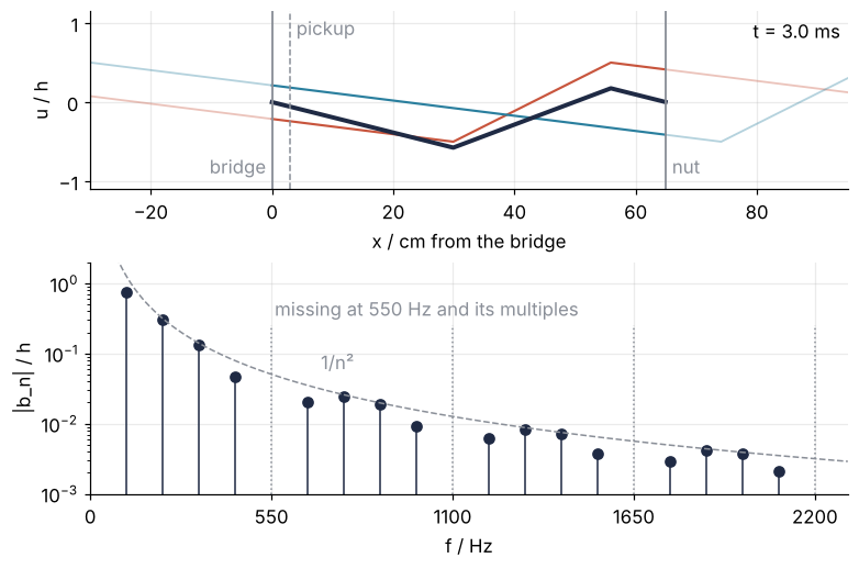
The upper panel is the string at 3.0 ms with the pickup marked 3 cm from the bridge, the one point whose motion the record holds. The peaks sit at whole multiples of 110 Hz, as the round trip demands. At 550, 1,100, 1,650, and 2,200 Hz the amplitude is below 1e-16 h, which is rounding. Everywhere else the weights read off the record agree with the formula to six decimal places and follow the \(1/n^2\) envelope. The raw peaks do not follow it. They carry the pickup factor, which climbs up to the eleventh harmonic and falls after it.

Where it shows up

The guitar string is the easiest place to watch the wave equation, but it governs anything whose acceleration grows with the curvature of a field.

• Seismology. P and S waves are the wave equation in rock, with \(c^2 = (\lambda + 2\mu)/\rho\) and \(c^2 = \mu/\rho\) for density \(\rho\), where \(\mu\) is the rock's stiffness against shear and \(\lambda + 2\mu\) its stiffness against compression in a P wave (\(\lambda\) and \(\mu\) are the Lamé parameters). In the upper crust they run at about 6 and 3.5 km/s, so the S wave falls behind by 11.9 s for every 100 km. That delay gives each station its distance from an earthquake, and three stations locate it.
• Organ pipes and the voice. The pressure in a pipe obeys the same equation, and a pipe open at both ends has every harmonic \(nc/2L\), like the string. Close one end and only the odd ones \((2n - 1)c/4L\) are left: the vocal tract, about 17 cm long and closed at the glottis, puts its resonances near 504, 1,513, and 2,522 Hz with sound at 343 m/s, its speed in dry air at 20 °C; the warmer air of the tract raises them a little.
• Light in a waveguide. Every component of the electromagnetic field obeys the wave equation, and the walls of a metal guide play the fixed ends. The lowest mode of a rectangular guide of width \(a\) has its cutoff at \(c/2a\), the string's \(f_1\) formula, which is 6.56 GHz for the 22.86 mm wide WR-90 guide.
• Stay cables of a bridge. A stay cable is a taut string, and engineers find its tension from its measured fundamental, \(\tau = 4\mu L^2 f_1^2\). A 100 m cable of 60 kg/m that swings at 1.2 Hz carries 3.46 MN.
• Water in a channel. Waves much longer than the depth \(d\) travel at \(\sqrt{gd}\), and a closed basin sloshes back and forth as a seiche with the period \(2L/\sqrt{gd}\), Merian's formula and the string's round trip again. A lake 10 km long and 50 m deep has a seiche of 15.1 min.

In each case the ends and the speed fix the frequencies, as whole multiples of one round trip, and the starting shape decides only how much of each.

Further reading

• numpy.fft for rfft and rfftfreq, and numpy.trapezoid for the weights.
• Fletcher and Rossing, The Physics of Musical Instruments, for strings and pipes as instruments use them.
• Strauss, Partial Differential Equations: An Introduction, for d'Alembert's solution and separation of variables, worked out in full.
• Related tutorials on this site: The Fourier transform: asking a signal how much of each frequency it contains, the spectrum; Plucked string harmonics: why a pluck at a third has no third harmonic, pull the string yourself and hear it; The wave equation with leapfrog finite differences: a pulse on a string, the same equation on a grid, with d'Alembert as the check; Finite differences: the heat equation as a matrix, and why the time step has a limit, the other classic equation; Sparse eigenvalues with scipy.sparse.linalg.eigsh: the tones of a drum, where the overtones are not whole multiples.
• Download the notebook. It was executed with the library versions in the header.