Richardson-Lucy deconvolution with scikit-image: two beads in one blur

The problem: two beads that look like one

Two fluorescent beads about 140 nm across lie 0.3 µm apart on a slide. Under a widefield microscope they show up as one elongated blob, because the microscope images every point as a small spot, its point spread function (PSF), here close to a Gaussian with a standard deviation of 0.25 µm. Microscopists quote the width of such a spot as its full width at half maximum (FWHM), the distance between the two points where it falls to half its peak. For any Gaussian that is 2.355 sigma (half height lies \(\sigma\sqrt{2\ln 2}\) from the center on either side), so 0.59 µm here. Two equal Gaussians only show a dip between them when they are more than 2 sigma apart, and these two are 1.2 sigma apart.

The image is the scene convolved with the PSF, the blur of the convolution tutorial, plus background light and photon noise. Deconvolution undoes the blur. With the PSF known, skimage.restoration.richardson_lucy iterates toward the scene that, once blurred, would explain the measurement. Run long enough, it splits the blob. Run too long, it turns the photon noise into detail that is not there and shrinks every bead to a spike.

The data are generated in Setup: the pair and four isolated beads on a 96 × 96 image with 0.05 µm pixels. The PSF is an exact Gaussian, which a real one never is, and the true scene is known, which with real data it is not. Step 4 shows how to stop without it.

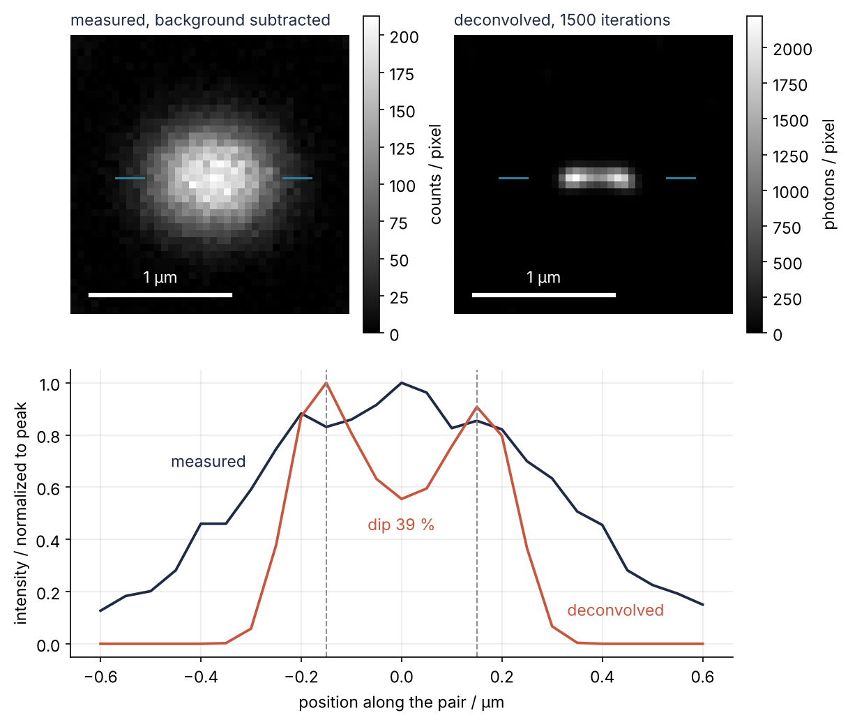
Step 6 draws it: the measured and the deconvolved image, and the profile through the pair, where the deconvolved curve dips 39 % below its lower peak.

Setup

One cell builds the PSF, a normalized 41 × 41 kernel, the true scene, and the measured image with Poisson noise from a fixed seed. Two helpers measure what the steps watch. dip is how far the row through the pair falls between its peaks, as a fraction of the lower one, so 0 means one blob. bead_fwhm is the FWHM defined above, averaged over the four isolated beads, with straight lines between pixels.

import numpy as np
import matplotlib.pyplot as plt
from scipy.signal import fftconvolve
from skimage.restoration import richardson_lucy

plt.rcParams.update({
    "figure.figsize": (7, 3.6), "figure.dpi": 110,
    "axes.spines.top": False, "axes.spines.right": False,
    "axes.grid": True, "grid.alpha": 0.25,
    "font.size": 11, "lines.linewidth": 1.8,
})
INK, ACCENT, SECOND, MUTED = "#1f2a44", "#c8553d", "#2a7f9e", "#8a8f98"

PIXEL = 0.05            # µm per pixel
PSF_SIGMA = 0.25        # µm, the microscope's blur
PHOTONS = 20_000        # per bead
BACKGROUND = 5.0        # photons per pixel
BEAD_SIGMA = 0.05       # µm, the spot drawn for each bead
BEAD_DIAMETER = 0.136   # µm, the sphere that spot stands for; your supplier's number goes here
rng = np.random.default_rng(0)

def gaussian_psf(sigma_um):
    half = round(4 * PSF_SIGMA / PIXEL)           # 20 pixels, so 41 x 41 for every width tried
    x = np.arange(-half, half + 1) * PIXEL
    kernel = np.exp(-(x[:, None] ** 2 + x[None, :] ** 2) / (2 * sigma_um ** 2))
    return kernel / kernel.sum()                  # sums to 1: the blur keeps the photon count

psf = gaussian_psf(PSF_SIGMA)
HALF = psf.shape[0] // 2

N = 96
PAIR_ROW, PAIR_COLS = 48, (45, 51)                # 6 pixels = 0.3 µm apart
SINGLES = [(20, 20), (20, 76), (76, 20), (76, 76)]
row, col = np.indices((N, N))

def bead(r, c):
    spot = np.exp(-((row - r) ** 2 + (col - c) ** 2) * PIXEL ** 2 / (2 * BEAD_SIGMA ** 2))
    return PHOTONS * spot / spot.sum()

truth = sum(bead(PAIR_ROW, c) for c in PAIR_COLS) + sum(bead(r, c) for r, c in SINGLES)
blurred = fftconvolve(truth, psf, mode="same") + BACKGROUND
measured = rng.poisson(blurred)
# Your data: measured = your image in counts, psf = a bead image cropped, background
# subtracted and divided by its sum, PIXEL = your pixel size; move PAIR_*, SINGLES,
# and the two peak windows in dip and in Step 6.

def dip(image):
    profile = image[PAIR_ROW]
    left = 40 + np.argmax(profile[40:48])         # each peak within 8 pixels of the center
    right = 49 + np.argmax(profile[49:57])
    return 1 - profile[left:right + 1].min() / min(profile[left], profile[right])

def bead_fwhm(image):
    widths = []
    for r, c in SINGLES:
        profile = image[r, c - 10:c + 11]
        k = np.argmax(profile)
        half = profile[k] / 2
        i = j = k
        while profile[i - 1] > half:
            i -= 1
        while profile[j + 1] > half:
            j += 1
        left = i - (profile[i] - half) / (profile[i] - profile[i - 1])
        right = j + (profile[j] - half) / (profile[j] - profile[j + 1])
        widths.append((right - left) * PIXEL)
    return np.mean(widths)

print(f"measured: {measured.shape}, {measured.dtype}, max {measured.max()} counts, dip {100 * dip(measured):.0f} %")
print(f"truth:    max {truth.max():,.0f} photons per pixel, bead FWHM {bead_fwhm(truth):.3f} µm")

measured: (96, 96), int64, max 218 counts, dip 0 %
truth:    max 3,183 photons per pixel, bead FWHM 0.123 µm

The blur spreads each bead's 20,000 photons so thin that the brightest measured pixel holds 218 counts, where the truth has 3,183.

Step 1: Subtract the background and keep floats

Richardson-Lucy corrects its estimate by multiplying it with ratios (Step 2 shows how), so it needs an image that is never negative and is zero where the sample sent no light. The 5 photons per pixel of background never passed through the PSF, so they come off first. Take the median of a strip 4 pixels wide along the border, where no bead sits. The median of the whole image would not do here, because six beads put more light into this small field than the background does.

frame = np.ones((N, N), dtype=bool)
frame[4:-4, 4:-4] = False
background = np.median(measured[frame])
image = np.clip(measured.astype(float) - background, 0, None)

print(f"background {background:.1f} counts (true {BACKGROUND:.0f}), median of the whole image {np.median(measured):.1f}")
print(f"pixels at zero: {100 * np.mean(image == 0):.0f} %, "
      f"{100 * np.mean(measured < background):.0f} % below the background and "
      f"{100 * np.mean(measured == background):.0f} % on it")

background 5.0 counts (true 5), median of the whole image 7.0
pixels at zero: 37 %, 25 % below the background and 12 % on it

The strip gives the true 5 counts, the whole image 7. After the subtraction 37 % of the pixels are zero: 25 % of the image read fewer than 5 counts and were clipped, and another 12 % read exactly 5, since photon counts are integers.

Show code

Copy

def show(ax, img, label, colorbar=True, unit="photons / pixel"):
    im = ax.imshow(img, cmap="gray")
    if colorbar:
        plt.colorbar(im, ax=ax, label=unit, shrink=0.85)
    h, w = img.shape
    x0, y0 = 0.06 * w, 0.92 * h
    ax.plot([x0, x0 + 1 / PIXEL], [y0, y0], color="white", lw=3)     # 1 µm scale bar
    ax.text(x0 + 0.5 / PIXEL, y0 - 0.03 * h, "1 µm", color="white", ha="center", va="bottom")
    ax.text(0, 1.02, label, transform=ax.transAxes, va="bottom", color=INK)
    ax.set_axis_off()

fig, axes = plt.subplots(1, 2, figsize=(7, 3.4), layout="constrained")
show(axes[0], truth, "truth")
show(axes[1], measured, "measured", unit="counts / pixel")
plt.show()

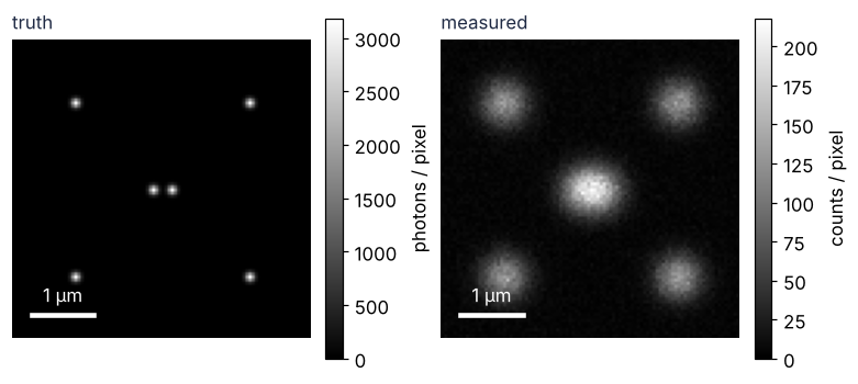
The pair is one blob, and each isolated bead is a soft disc about as wide as the PSF.

Step 2: Deconvolve with richardson_lucy

Richardson-Lucy starts from a flat guess, 0.5 everywhere in scikit-image, and repeats one correction. Blur the guess with the PSF, which gives the image the guess would produce, and divide the measured image by it. Where the guess explains too little light, the ratio is above 1. Blur the ratio with the PSF flipped (a Gaussian is unchanged by the flip) and multiply the guess by the result:

with \(u_k\) the estimate after \(k\) iterations, \(d\) the measured image, \(P\) the PSF, and \(*\) convolution. The guess grows where light is missing and shrinks where it has too much.

The blur inside richardson_lucy treats everything beyond the border as black. Near the edge the blurred guess comes out too dark, the ratio comes out above 1, and the iterations pile light into a bright ridge just inside the border. Padding the image by the PSF's half-width with a mirrored copy gives the blur plausible light to find, and cropping afterwards removes it. np.pad(..., mode="symmetric") is NumPy's name for the mirroring that SciPy calls "reflect" in the convolution tutorial. NumPy's own "reflect" leaves out the edge pixel, which makes no visible difference behind a 41-pixel PSF.

def deconvolve(image, psf, n):
    h = psf.shape[0] // 2
    padded = np.pad(image, h, mode="symmetric")
    return richardson_lucy(padded, psf, num_iter=n, clip=False)[h:-h, h:-h]

estimate = deconvolve(image, psf, 100)
print(f"total      {image.sum():9,.0f} -> {estimate.sum():9,.0f} photons")
print(f"maximum    {image.max():9,.0f} -> {estimate.max():9,.0f} photons")
print(f"bead FWHM  {bead_fwhm(image):9.2f} -> {bead_fwhm(estimate):9.2f} µm")
print(f"dip        {100 * dip(image):7.0f} % -> {100 * dip(estimate):7.0f} %")

total        124,141 ->   124,519 photons
maximum          213 ->     1,257 photons
bead FWHM       0.56 ->      0.19 µm
dip              0 % ->       0 %

clip=False keeps the counts; the first Pitfall says why.

After 100 iterations the total is the same to 0.3 %, but the light has gathered: the brightest pixel went from 213 to 1,257 photons and the isolated beads shrank from 0.56 to 0.19 µm. The pair is still one blob. Sharper, not yet split.

Step 3: Follow the error over the iterations

Because the truth is known here, you can measure how far each result is from it: the root of the mean squared pixel difference (RMS error), divided by the brightest true pixel. richardson_lucy cannot resume where it stopped, so each count runs from scratch, about 10,000 iterations in all.

counts = [10, 30, 100, 200, 300, 500, 700, 1000, 1500, 2000, 3000]
estimates = {n: deconvolve(image, psf, n) for n in counts}

def rms_error(estimate):
    return np.sqrt(np.mean((estimate - truth) ** 2)) / truth.max()

n_best = min(counts, key=lambda n: rms_error(estimates[n]))
print("iterations     error      dip")
for n in counts:
    print(f"{n:10d}  {100 * rms_error(estimates[n]):6.2f} %  {100 * dip(estimates[n]):5.0f} %")

iterations     error      dip
        10    3.80 %      0 %
        30    3.36 %      0 %
       100    2.70 %      0 %
       200    2.23 %      0 %
       300    1.95 %      0 %
       500    1.62 %      3 %
       700    1.45 %     12 %
      1000    1.37 %     25 %
      1500    1.49 %     39 %
      2000    1.74 %     49 %
      3000    2.31 %     61 %

The error falls to 1.37 % at 1,000 iterations and climbs back to 2.31 % at 3,000. The pair starts to split at 500, and its dip keeps deepening past the minimum, to 61 % at 3,000.

Show code

Copy

fig = plt.figure(figsize=(7, 5.6), layout="constrained")
axs = fig.subplot_mosaic([["err", "err", "err"], ["a", "b", "c"]], height_ratios=[1, 1.1])
ax = axs["err"]
ax.plot(counts, [100 * rms_error(estimates[n]) for n in counts], "o-", color=ACCENT, ms=4)
ax.axvline(n_best, color=MUTED, ls="--", lw=1)
ax.text(n_best * 1.1, 3.4, f"minimum at {n_best}", color=MUTED, va="top")
ax.set(xscale="log", xlabel="iterations", ylabel="RMS error / % of peak")
center = slice(32, 64)                            # the central 1.6 µm
for key, n in zip("abc", [30, n_best, 3000]):
    show(axs[key], estimates[n][center, center], f"{n} iterations", colorbar=False)
plt.show()

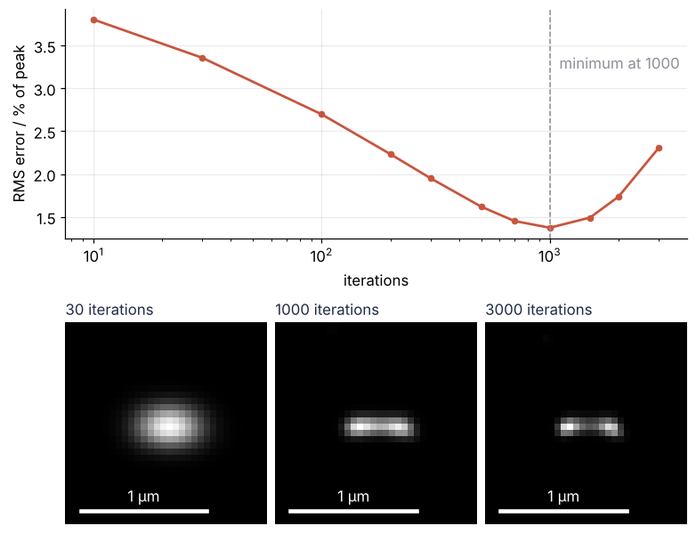
At 30 iterations the pair is a round blob. At 1,000 it is a short bar with a bright spot at each end. At 3,000 the bar is shorter and its middle dimmer, and Step 4 shows that by then the beads are smaller than they really are.

Late iterations hurt because the blur smooths fine detail away: a scene with a fine, rapid pattern blurs to almost the same image as one without it. Each iteration adds finer detail to the estimate, and the finest detail the data hold is about as weak as the noise. Past some count the iterations explain the noise's random pixel-to-pixel wiggle as blurred light, and the blur makes that costly:

stripes = np.cos(2 * np.pi * col * PIXEL / 0.5)   # stripes 0.5 µm apart, height 1
kept = np.ptp(fftconvolve(stripes, psf, mode="same")[PAIR_ROW, 30:66]) / 2
print(f"after the blur: height {kept:.4f}, so a wiggle needs stripes {1 / kept:.0f} times taller")

after the blur: height 0.0072, so a wiggle needs stripes 139 times taller

Stripes 0.5 µm apart come through at 0.7 % of their height. To explain a noise wiggle of that spacing, the estimate needs stripes 139 times taller. The condition number tutorial has the general case: a small change in the data, a large change in the answer.

Anything that keeps a method from fitting the noise, usually by preferring the smoother answer, is called regularization. richardson_lucy has none built in, so stopping early is its regularization and the iteration count its knob. The fall and rise of the error is called semi-convergence. SART, the iterative method in CT reconstruction with scikit-image, does the same.

Step 4: Choose the iteration count without the truth

Real data have no error curve, but two things they do give stand in for it.

The first is the residual. A photon count with Poisson noise has a variance equal to its mean, so a pixel expected to hold 100 counts scatters by about 10. Blur the estimate and add the background back: that is the model \(m\) of every pixel's counts. The mean of \((d - m)^2 / m\) falls to about 1 once the model explains all but the noise, and the discrepancy rule stops at the first count where it does. The PSF must sum to 1 for this.

The second is a bead image: beads of known size below the resolution, here the four isolated beads. A uniform sphere seen from above falls to half its central brightness at 0.87 of its diameter, so stop where the beads reach 0.87 times the supplier's diameter. A 100 nm bead gives 0.087 µm, under two pixels at 0.05 µm, too few to read.

def blur(estimate, psf):
    h = psf.shape[0] // 2
    return fftconvolve(np.pad(estimate, h, mode="symmetric"), psf, mode="valid")

def residual(estimate):
    model = blur(estimate, psf) + background
    return np.mean((measured - model) ** 2 / model)

target = 0.87 * BEAD_DIAMETER
widths = {n: bead_fwhm(estimates[n]) for n in counts}
N_FIT = next(n for n in counts if residual(estimates[n]) <= 1)    # the discrepancy rule
N_ITER = next(n for n in counts if widths[n] <= target)             # the bead rule

print(f"target {target:.3f} µm, Gaussian spot FWHM {2.355 * BEAD_SIGMA:.3f} µm")
print("iterations  residual  bead FWHM / µm")
for n in counts:
    print(f"{n:10d}  {residual(estimates[n]):8.3f}  {widths[n]:14.3f}")
print(f"N_FIT = {N_FIT}, N_ITER = {N_ITER}, error {100 * rms_error(estimates[N_ITER]):.2f} %; smallest error at {n_best}")

# could the residual tell the two stops apart? only if their models differ by more than the noise
model_fit = blur(estimates[N_FIT], psf) + background
change = np.abs(blur(estimates[N_ITER], psf) + background - model_fit) / np.sqrt(model_fit)
print(f"largest change of the model from {N_FIT} to {N_ITER} iterations: {change.max():.2f} noise sigma")

target 0.118 µm, Gaussian spot FWHM 0.118 µm
iterations  residual  bead FWHM / µm
        10     1.398           0.356
        30     1.084           0.261
       100     1.004           0.193
       200     0.989           0.167
       300     0.985           0.155
       500     0.981           0.141
       700     0.980           0.133
      1000     0.979           0.124
      1500     0.978           0.115
      2000     0.978           0.108
      3000     0.978           0.098
N_FIT = 200, N_ITER = 1500, error 1.49 %; smallest error at 1000
largest change of the model from 200 to 1500 iterations: 0.40 noise sigma

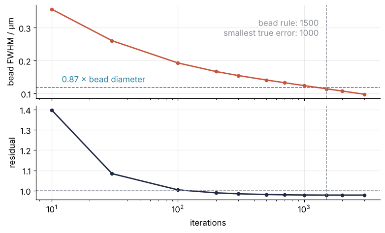
The residual drops below 1 at 200 iterations, with the pair still one blob. That stop is safe but early, and the residual cannot do better: from 200 to 1,500 iterations the model changes by at most 0.40 of the noise in any pixel.

The bead rule picks 1,500, one count past the smallest error, at 1.49 % against 1.37 %. It runs long because bead_fwhm reads even the true scene as 0.123 µm, above the 0.118 µm target, so the estimate must become narrower than the truth.

Cells come without beads. Image a bead slide with the same objective, pixel size, and exposure, its beads about as bright as your sample's brightest structures: the right count depends on the photon count, and brighter beads tolerate more iterations than a dimmer sample. On the sample itself the discrepancy rule still gives the lower bound.

Show code

Copy

fig, (ax1, ax2) = plt.subplots(2, 1, figsize=(7, 4.2), sharex=True, layout="constrained")
ax1.plot(counts, [widths[n] for n in counts], "o-", color=ACCENT, ms=4)
ax1.axhline(target, color=SECOND, ls="--", lw=1)
ax1.text(12, target + 0.01, "0.87 × bead diameter", color=SECOND, va="bottom")
ax1.text(N_ITER / 1.15, 0.33, f"bead rule: {N_ITER}\nsmallest true error: {n_best}", color=MUTED, ha="right", va="top")
ax1.set(ylabel="bead FWHM / µm")
ax2.plot(counts, [residual(estimates[n]) for n in counts], "o-", color=INK, ms=4)
ax2.axhline(1, color=MUTED, ls="--", lw=1)
ax2.set(xscale="log", xlabel="iterations", ylabel="residual")
for ax in (ax1, ax2):
    ax.axvline(N_ITER, color=MUTED, ls="--", lw=1)
plt.show()

Step 5: Check what a wrong PSF width does

A PSF taken from a formula or a bead image is never exact. Deconvolve at N_ITER with widths 10 % and 20 % off on either side:

print("PSF sigma / µm     error      dip   max / photons")
for sigma in [0.20, 0.225, 0.25, 0.275, 0.30]:
    est = deconvolve(image, gaussian_psf(sigma), N_ITER)
    print(f"{sigma:14.3f}  {100 * rms_error(est):6.2f} %  {100 * dip(est):5.0f} %  {est.max():14,.0f}")

PSF sigma / µm     error      dip   max / photons
         0.200    4.00 %     16 %             443
         0.225    3.42 %     33 %             730
         0.250    1.49 %     39 %           5,026
         0.275    9.10 %      0 %          15,953
         0.300   13.24 %      0 %          19,589

Too narrow leaves part of the blur in: at 0.20 µm the error is 4.00 % against 1.49 %, and the pair still splits, if less. Too wide is worse. At 0.275 µm the pair merges again and the error is six times larger, and at 0.30 µm the pair collapses into a single spike of 19,589 photons, six times the true bead's peak. When unsure, err toward the narrower PSF, and measure it from a bead image.

Step 6: Show the pair before and after

The final figure sets the measured image beside the deconvolved one at N_ITER and draws the profile along the row through the pair, each curve scaled to its own maximum.

Show code

Copy

final = estimates[N_ITER]
fig = plt.figure(figsize=(8, 7), layout="constrained")
axs = fig.subplot_mosaic([["m", "d"], ["p", "p"]], height_ratios=[1.3, 1])
crop = slice(28, 68)                              # the central 2 µm around the pair
show(axs["m"], image[crop, crop], "measured, background subtracted", unit="counts / pixel")
show(axs["d"], final[crop, crop], f"deconvolved, {N_ITER} iterations")
for key in "md":                                  # ticks at the ends of the profile row
    for c0 in (34 - 28, 58 - 28):
        axs[key].plot([c0, c0 + 4], [PAIR_ROW - 28, PAIR_ROW - 28], color=SECOND, lw=1.5)

cols = np.arange(36, 61)
x_um = (cols - 48) * PIXEL
ax = axs["p"]
ax.plot(x_um, image[PAIR_ROW, cols] / image[PAIR_ROW, cols].max(), color=INK)
ax.plot(x_um, final[PAIR_ROW, cols] / final[PAIR_ROW, cols].max(), color=ACCENT)
ax.text(-0.31, 0.70, "measured", color=INK, ha="right", va="center")       # each curve named beside it
ax.text(0.33, 0.13, "deconvolved", color=ACCENT, ha="left", va="center")
for xb in (-0.15, 0.15):
    ax.axvline(xb, color=MUTED, ls="--", lw=1)
ax.text(0, final[PAIR_ROW, 48] / final[PAIR_ROW, cols].max() - 0.06, f"dip {100 * dip(final):.0f} %",
        color=ACCENT, ha="center", va="top")
ax.set(xlabel="position along the pair / µm", ylabel="intensity / normalized to peak")
plt.show()

peaks = [40 + np.argmax(final[PAIR_ROW, 40:48]), 49 + np.argmax(final[PAIR_ROW, 49:57])]
print(f"dip {100 * dip(final):.0f} %, peaks {(peaks[1] - peaks[0]) * PIXEL:.2f} µm apart (true 0.30 µm)")

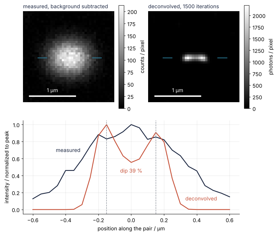
dip 39 %, peaks 0.30 µm apart (true 0.30 µm)

The measured profile is a single hump. The deconvolved one dips 39 % below its lower peak, and its maxima sit 0.30 µm apart, on the true positions. One noise draw proves little, so here are five more of the same scene, each treated as in Steps 1 and 2:

dips = []
for _ in range(5):
    draw = rng.poisson(blurred)
    img = np.clip(draw.astype(float) - np.median(draw[frame]), 0, None)
    dips.append(dip(deconvolve(img, psf, N_ITER)))
print("dips:", "  ".join(f"{100 * d:.0f} %" for d in dips))

dips: 42 %  0 %  26 %  21 %  41 %

Four of the five split, with dips from 21 % to 42 %, and one stays a single blob. At 20,000 photons per bead a pair 0.3 µm apart splits in most draws, not all. More photons let the iterations run longer before the noise wins.

Pitfalls

The numbers below come from this cell, run at N_ITER:

h = HALF
default = richardson_lucy(np.pad(image, h, mode="symmetric"), psf, num_iter=N_ITER)[h:-h, h:-h]
scaled = richardson_lucy(np.pad(image / image.max(), h, mode="symmetric"), psf, num_iter=N_ITER)[h:-h, h:-h]
print(f"clip=True:          max {default.max():.2f}, total {100 * default.sum() / image.sum():.1f} % of the input, "
      f"dip {100 * dip(default):.0f} %; input scaled to 1: max {scaled.max():.2f}, dip {100 * dip(scaled):.0f} %")
left_in = deconvolve(measured.astype(float), psf, N_ITER) - background
print(f"background left in: error {100 * rms_error(left_in):.2f} % against {100 * rms_error(final):.2f} %, dip {100 * dip(left_in):.0f} %")
print(f"uint16 arithmetic:  [3, 200] - 5 = {np.array([3, 200], dtype=np.uint16) - 5}")

edge_truth = truth + bead(PAIR_ROW, 1)            # a bead cut by the left border
edge_image = np.clip(rng.poisson(fftconvolve(edge_truth, psf, mode="same") + BACKGROUND) - background, 0, None)
for name, est in [("padded", deconvolve(edge_image, psf, N_ITER)),
                  ("not padded", richardson_lucy(edge_image, psf, num_iter=N_ITER, clip=False))]:
    err = np.sqrt(np.mean((est - edge_truth) ** 2)) / edge_truth.max()
    print(f"edge bead, {name:10s}  peak {est[40:57, :6].max():6,.0f} (true {edge_truth[PAIR_ROW, 1]:,.0f}), error {100 * err:.2f} %")

clip=True:          max 1.00, total 1.0 % of the input, dip 0 %; input scaled to 1: max 1.00, dip 0 %
background left in: error 2.11 % against 1.49 %, dip 2 %
uint16 arithmetic:  [3, 200] - 5 = [65534   195]
edge bead, padded      peak  2,323 (true 3,381), error 2.01 %
edge bead, not padded  peak  5,142 (true 3,381), error 3.07 %

The default clip=True. The result comes out flat and washed out, with a maximum of exactly 1.00, a total of 1.0 % of the input, and no pair. clip=True cuts every value above 1 and below -1, a convention for images scaled to that range, and an image in counts lives far above it. Scaling the input to a maximum of 1 does not save it, because the deconvolved peaks rise far above the measured maximum, and the scaled run still shows no dip. Pass clip=False every time.

Background left in, or subtracted from an unsigned image. Leave the 5 counts in and the pair barely splits at 1,500 iterations, a dip of 2 % against 39 %, with an error of 2.11 % against 1.49 %: the iterations spend their effort explaining a flat floor they cannot sharpen. Subtract the background from a camera's uint16 image and the dark pixels wrap around, since 3 − 5 is 65,534 in that type. Step 1's line converts to float first, then subtracts and clips. An integer image on its own is harmless, because richardson_lucy converts it to float.

Edges. A bead cut by the frame, deconvolved without padding, collapses into a spike of 5,142 photons where the truth peaks at 3,381, and the error over the image grows by half, 3.07 % against 2.01 %. The cause is the black beyond the border from Step 2, and the fix is Step 2's symmetric padding. Even padded, the cut bead peaks at only 2,323, because the mirrored copy is a guess too. Trust nothing within a PSF half-width of the border.

Variations

• A measured PSF. Crop 41 × 41 pixels around each isolated bead of a bead image, subtract the background, average the crops, divide by the sum, and pass the result as psf.
• A 3D stack. richardson_lucy takes n-dimensional arrays. Pass a z-stack and a 3D PSF, which is stretched along the optical axis: about 2.6 times its lateral width for an oil objective at NA 1.4, about seven times at the NA of 0.45 that a 0.59 µm spot implies in green light. Expect the run time to grow with the number of voxels.
• One step instead of many. skimage.restoration.wiener, with a balance parameter, or unsupervised_wiener deconvolve in one linear step, with negative values and ringing where Richardson-Lucy stays non-negative.
• Denoise first. Run a mild denoising filter from Denoise a low-light micrograph with scikit-image before the deconvolution.

Cheat sheet

image = np.clip(measured.astype(float) - background, 0, None)   # float first, then subtract, clip at 0
psf = psf / psf.sum()                                            # sum 1, needed for the residual
h = psf.shape[0] // 2
padded = np.pad(image, h, mode="symmetric")                      # mirror the border, crop afterwards
est = richardson_lucy(padded, psf, num_iter=n, clip=False)[h:-h, h:-h]   # clip=True caps at 1
model = fftconvolve(np.pad(est, h, mode="symmetric"), psf, mode="valid") + background
residual = np.mean((measured - model) ** 2 / model)             # about 1 for Poisson counts; stops early
# stop where isolated beads reach FWHM = 0.87 x bead diameter, at least two pixels wide

Further reading

• The scikit-image API page of skimage.restoration, for richardson_lucy, wiener, and unsupervised_wiener, and the gallery example Image Deconvolution.
• Richardson, "Bayesian-based iterative method of image restoration", Journal of the Optical Society of America 62 (1972), 55-59; Lucy, "An iterative technique for the rectification of observed distributions", Astronomical Journal 79 (1974), 745-754.
• Bertero and Boccacci, Introduction to Inverse Problems in Imaging (IOP Publishing, 1998), for semi-convergence and the stopping rules of iterative methods.
• Related tutorials on this site: Convolution: how a small kernel blurs, sharpens, and finds edges; CT reconstruction with scikit-image: a head slice from its projections; Denoise a low-light micrograph with scikit-image: what each filter keeps; Background subtraction: one threshold for every cell in a microscope image; The condition number: how many digits a linear solve can lose; The Fourier transform: asking a signal how much of each frequency it contains, for the frequency view of why late iterations amplify noise.
• Download the notebook. It was executed with the library versions in the header.