Filtered back projection: why the ramp filter sharpens a CT slice (Python)

The question

A CT scanner, or a micro-CT at a synchrotron beamline, is calibrated with small dense beads. Put one bead of 9 pixels into a 256-pixel slice, 64 px from the rotation axis, and let the scanner measure 180 parallel projections over half a turn. Each projection is one column of the sinogram on the left. Smear every projection back across the slice along its rays, add up the 180 smears, and you get the image on the right. Filtered back projection, the method CT scanners ran on for decades, does the same with one change: a ramp filter applied to every projection first.

Show code

import warnings
import numpy as np
import matplotlib.pyplot as plt
from matplotlib.colors import PowerNorm

warnings.filterwarnings("ignore", message="IProgress not found")   # skimage.data warns about a missing progress widget
from skimage.data import shepp_logan_phantom
from skimage.transform import radon, iradon, rescale

plt.rcParams.update({
    "figure.figsize": (8, 3.4), "figure.dpi": 110,
    "axes.spines.top": False, "axes.spines.right": False,
    "axes.grid": True, "grid.alpha": 0.25,
    "font.size": 11, "lines.linewidth": 1.8,
})
INK, ACCENT, SECOND, MUTED = "#1f2a44", "#c8553d", "#2a7f9e", "#8a8f98"

N = 256
row, col = np.indices((N, N))
x, y = col - N // 2, N // 2 - row                  # px, x to the right, y up, origin on the rotation axis
inside = np.hypot(x, y) < N / 2                    # the disk every angle sees

bead_row, bead_col = N // 2 - 40, N // 2 + 50
bead = (np.hypot(row - bead_row, col - bead_col) <= 1.5).astype(float)
r = np.hypot(col - bead_col, row - bead_row)       # distance from the bead, px

theta = np.linspace(0, 180, 180, endpoint=False)   # degrees
sino = radon(bead, theta)
plain = iradon(sino, theta, filter_name=None)

track = sino.argmax(axis=0)
near = plain[r <= 3].sum() / plain[inside].sum()
print(f"bead: {bead.sum():.0f} pixels, {np.hypot(40, 50):.1f} px from the axis")
print(f"track on the detector: {track.min()} to {track.max()} px, center {N // 2} px")
print(f"plain back projection: {100 * near:.1f} % of the signal within 3 px of the bead")

fig, (ax1, ax2) = plt.subplots(1, 2, figsize=(8, 3.4), width_ratios=[1.4, 1])
ax1.imshow(sino, cmap="gray", aspect="auto", extent=(0, 180, N, 0))
ax1.set(xlabel="θ / degrees", ylabel="detector position / px")
ax1.grid(False)
ax2.imshow(plain, cmap="gray", norm=PowerNorm(0.4, vmin=0))
ax2.plot(bead_col, bead_row, "o", ms=18, mfc="none", mec=SECOND, mew=1.8)
ax2.text(4, 6, f"{100 * near:.1f} % within 3 px", color="white", va="top")
ax2.set_axis_off()
plt.show()

bead: 9 pixels, 64.0 px from the axis
track on the detector: 78 to 192 px, center 128 px
plain back projection: 2.4 % of the signal within 3 px of the bead

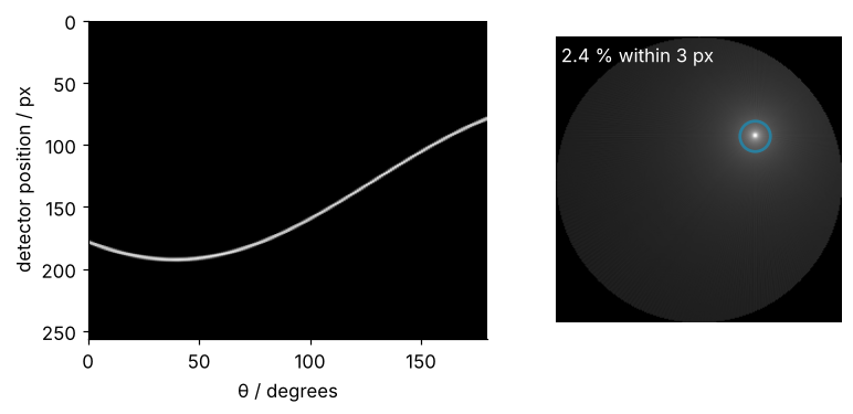
Left: sinogram of one bead, detector position in px against projection angle from 0 to 180 degrees; the bead traces a sine between 78 and 192 px. Right: its plain back projection on a power-law gray scale, a bright point at the true position (blue-green circle) inside a halo that fills the slice.

Two things are plain. The bead traces a sine across the sinogram, and that sine is where the sinogram has its name. Its crest lies at 192 px on a detector centered at 128 px, 64 px off center, which is the bead's distance from the axis. The trough would lie 64 px off on the other side, but it falls after 180°: half a turn ends at 78 px, 50 px off. And the smeared-back image has a bright point exactly where the bead is.

The rest is not plain. The bright point sits inside a halo that reaches the edge of the slice, and only 2.4 % of the back-projected signal lies within 3 px of the bead. Why does honest smearing put the material everywhere, and why does one particular filter, multiplying each projection's spectrum by its absolute frequency \(|k|\), remove the halo exactly?

The idea: smear every projection back along its rays

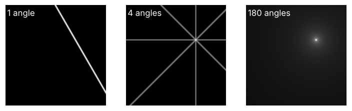
A projection tells you how much material lies on each ray, not where along the ray it sits. The fairest guess spreads each value evenly along its ray. Back projection does this for every angle and adds the results. Here is the bead back-projected from one angle, from four, and from all 180, with a back projection written by hand in a dozen lines of NumPy:

Show code

def backproject(sino, theta):
    """Spread every projection evenly along its rays and add up, scaled as iradon scales."""
    s_detector = np.arange(sino.shape[0]) - sino.shape[0] // 2
    image = np.zeros((N, N))
    for p, th in zip(sino.T, np.deg2rad(theta)):
        s = x * np.cos(th) + y * np.sin(th)        # where each pixel's ray hits the detector
        image += np.interp(s, s_detector, p, left=0, right=0)
    return image * np.pi / (2 * len(theta))


picks = {"1 angle": [30], "4 angles": [0, 45, 90, 135], "180 angles": list(range(180))}
smears = {label: backproject(sino[:, i], theta[i]) for label, i in picks.items()}

fig, axes = plt.subplots(1, 3, figsize=(8, 2.9))
for ax, (label, image) in zip(axes, smears.items()):
    ax.imshow(image, cmap="gray", norm=PowerNorm(0.5, vmin=0))
    ax.text(4, 6, label, color="white", va="top")
    ax.set_axis_off()
plt.show()

mismatch = np.abs(smears["180 angles"] - plain)[inside].max() / plain.max()
print(f"hand-written against iradon: largest difference {mismatch:.0e} of the peak")
for R in [10, 20, 40, 60]:
    ring = np.abs(r - R) < 0.5
    print(f"r = {R:2d} px:   r × value = {R * plain[ring].mean():.2f}")

The bead back-projected from 1 angle, 4 angles, and 180 angles, gray scale, each panel on its own scale: a single stripe at 30 degrees, a four-pointed star of stripes crossing at the bead, and a smooth halo around a bright center.

hand-written against iradon: largest difference 4e-16 of the peak
r = 10 px:   r × value = 4.48
r = 20 px:   r × value = 4.51
r = 40 px:   r × value = 4.50
r = 60 px:   r × value = 4.50

One angle gives a stripe. Four give a star of stripes that cross only at the bead, so the bead is already the brightest point. With 180 the stripes are so dense that they merge into a smooth halo around a bright center. The hand-written version agrees with scikit-image's iradon to rounding.

The halo falls off as \(1/r\), and the reason is counting. Every stripe is about as wide as the bead and passes through it. At a distance \(r\) from the bead, neighboring stripes are \(r\) times the angle step apart, so the number of stripes that cover a given pixel there falls as \(1/r\). The printed rings check it: \(r\) times the back-projected value is 4.48 at 10 px and 4.50 at 60 px, a constant to within 1 %. A \(1/r\) halo is a strange object: a ring at radius \(r\) is \(2\pi r\) long, so every ring holds the same signal, and the signal inside a circle of radius \(R\) grows in proportion to \(R\). There is no radius at which most of it has been collected; the slice simply ends first.

Each stripe has one property that matters for what follows: it is constant along its rays, and that makes it simple in Fourier space.

Lines through the center: the Fourier slice theorem

One smear is one line. A point \((k_x, k_y)\) of an image's 2D Fourier transform stands for a stripe pattern across the image, with the direction and spacing that point encodes, as in MRI k-space. Every stripe pattern that varies along a smear's rays averages to zero against it, and only patterns that vary across the rays survive. Their wave vectors all point along the detector, so they lie on one line through the origin of Fourier space, at the angle of the projection.

Show code

k = np.fft.fftfreq(N)                              # cycles per pixel
kx, ky = np.meshgrid(k, -k)                        # rows run downward, y runs up


def power_near_line(image, angle):
    """Fraction of the image's spectral power within 3 Fourier pixels of the line at this angle."""
    power = np.abs(np.fft.fft2(image))**2
    th = np.deg2rad(angle)
    off_line = np.abs(-kx * np.sin(th) + ky * np.cos(th)) * N
    return power[off_line <= 3].sum() / power.sum()


for angle in [0, 30]:
    one_smear = backproject(sino[:, [angle]], theta[[angle]])
    print(f"single smear at {angle:2d}°: {100 * power_near_line(one_smear, angle):.0f} % of the power on its line")

phantom = rescale(shepp_logan_phantom(), N / 400, anti_aliasing=True) * inside
sino_phantom = radon(phantom, theta)


def slice_check(angle):
    """1D transform of one projection, and the 2D transform of the slice summed along that line."""
    th = np.deg2rad(angle)
    P = np.fft.fft(np.fft.ifftshift(sino_phantom[:, angle]))     # detector center to index 0
    s = (x * np.cos(th) + y * np.sin(th)).ravel()
    F_line = np.array([np.sum(phantom.ravel() * np.exp(-2j * np.pi * q * s)) for q in k])
    return P, F_line


for angle in [0, 30]:
    P, F_line = slice_check(angle)
    print(f"slice theorem at {angle:2d}°: largest deviation {np.abs(P - F_line).max() / np.abs(F_line).max():.2g}")
P30, F30 = P, F_line                               # the 30° line, plotted on the right

fig, axes = plt.subplots(1, 3, figsize=(8, 2.9), width_ratios=[1, 1, 1.25])
edge = (-0.5, 0.5, -0.5, 0.5)
for ax, image, decades in zip(axes[:2], [one_smear, phantom], [3, 4]):
    log_spectrum = np.log10(np.abs(np.fft.fftshift(np.fft.fft2(image))) + 1e-12)
    ax.imshow(log_spectrum, cmap="gray", extent=edge, vmin=log_spectrum.max() - decades)
    ax.set(xlabel="kx / cycles per px", xticks=[-0.5, 0, 0.5], yticks=[-0.5, 0, 0.5])
    ax.grid(False)
axes[0].set_ylabel("ky / cycles per px")
q = np.array([-0.5, 0.5])
for angle in range(0, 180, 15):                     # 12 of the 180 lines, the 30° line heavier
    th = np.deg2rad(angle)
    axes[1].plot(q * np.cos(th), q * np.sin(th), color=SECOND, lw=1.6 if angle == 30 else 0.8)
for ax in axes[:2]:
    ax.set(xlim=(-0.5, 0.5), ylim=(-0.5, 0.5))
positive = (k > 0) & (k < 0.5)
axes[2].semilogy(k[positive], np.abs(P30[positive]), color=INK)
axes[2].semilogy(k[positive][::4], np.abs(F30[positive][::4]), "o", ms=4, color=SECOND)
axes[2].set(xlabel="k / cycles per px", ylabel="|transform| / arb. units")
axes[2].text(0.10, 300, "2D, on the line", color=SECOND)                 # named in place, above the dots
axes[2].text(0.10, 1.5, "1D, projection", color=INK)                     # and below the curve
fig.tight_layout()
plt.show()

single smear at  0°: 100 % of the power on its line
single smear at 30°: 97 % of the power on its line
slice theorem at  0°: largest deviation 1.7e-15
slice theorem at 30°: largest deviation 0.0012

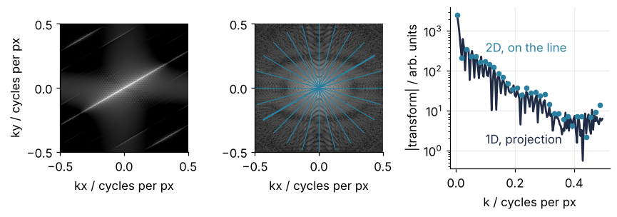
Left: 2D spectrum of the bead smeared back from the single 30-degree projection, nearly all of it on one line through the origin. Middle: spectrum of the head phantom with 12 of the 180 sampled lines, crowded at the center, the 30-degree line heavier. Right: the 1D spectrum of the phantom's 30-degree projection (line) against frequency matches the 2D spectrum along that line (dots).

At 0° the smear lies along the pixel grid and all of its power sits on the line. At 30° 97 % of it lies within 3 Fourier pixels of the line, a Fourier pixel being the spacing of the FFT's frequencies, 1/256 cycles per pixel here. The left panel shows the same: one bright line through the origin. The line is a few Fourier pixels wide there because the smear stops at the edge of the image.

What lies on the line. Along that line the smear's spectrum varies exactly as the projection varies along the detector, so the values on the line are the projection's 1D Fourier transform. They are also the slice's 2D transform on that line. The 1D transform weights each ray's sum with a wave \(e^{-2\pi i k s}\) that depends only on the detector position \(s\), so it is constant along the ray. Weighting the sum is then the same as weighting every point of the slice on that ray before summing: the slice times a 2D wave that runs across the rays, summed over the whole slice, which is the 2D transform at \((k\cos\theta, k\sin\theta)\). That is the Fourier slice theorem: the 1D transform of a projection at angle \(\theta\) is a cut through the 2D transform of the slice at the same angle.

The printed check runs it on the head phantom. At 0° the projection is a plain column sum and the two agree to rounding, a relative deviation of 1.7e-15. At 30° the deviation is 0.0012, or 0.12 %, which is the interpolation inside radon. The right panel compares them along the whole line.

The crowding. Back projection adds 180 such lines with equal weight, and they all pass through the origin. At a distance \(|k|\) from the origin neighboring lines are \(\pi |k| / 180\) apart, so the samples are dense at the center and sparse far out, with a density that falls as \(1/|k|\). The middle panel shows a dozen of the 180 lines on the phantom's spectrum. Their sum is the true spectrum times a weight that falls as \(1/|k|\): low frequencies come in far too strong, which is a blur. Weight every projection's spectrum by \(|k|\) first, the ramp, and the density evens out.

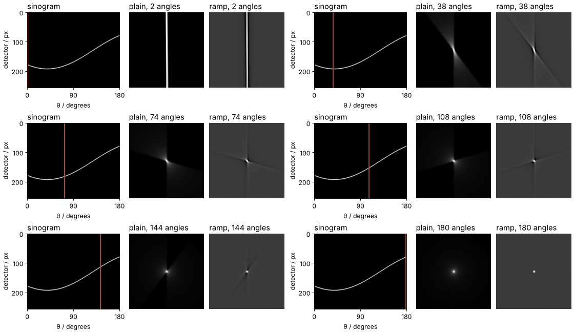
Watch the two sums build up angle by angle, the plain smears in the middle and the ramp-filtered ones on the right:

Animation over 180 angles. Left: the sinogram with the current angle marked. Middle: the plain smears add up to a halo around the bead. Right: the ramp-filtered smears, each with dark negative side lobes, cancel everywhere except at the bead.

Show code

"""Back projection angle by angle: plain smears pile up into a halo, ramp-filtered smears cancel.

Renders ../../assets/backprojection-accumulate.gif. Run it from any directory:

    python scene.py
"""
from pathlib import Path
import warnings

import numpy as np
import matplotlib.pyplot as plt
from matplotlib.animation import FuncAnimation, PillowWriter
from PIL import Image

warnings.filterwarnings("ignore", message="IProgress not found")
from skimage.transform import radon, iradon

OUT = Path(__file__).resolve().parents[2] / "assets" / "backprojection-accumulate.gif"
INK, ACCENT = "#1f2a44", "#c8553d"
plt.rcParams.update({"font.size": 11})

# ---- data: the bead of the tutorial and its sinogram
N = 256
row, col = np.indices((N, N))
bead_row, bead_col = N // 2 - 40, N // 2 + 50
bead = (np.hypot(row - bead_row, col - bead_col) <= 1.5).astype(float)
theta = np.linspace(0, 180, 180, endpoint=False)
sino = radon(bead, theta)

# ---- one smear per angle, plain and ramp-filtered, then running sums
# iradon of a single column scales by pi/2; dividing by 180 makes the sum equal iradon of all columns
def smear(i, filter_name):
    return iradon(sino[:, [i]], theta[[i]], filter_name=filter_name) / len(theta)

crop = np.s_[bead_row - 64:bead_row + 64, bead_col - 64:bead_col + 64]
plain_sum = np.cumsum([smear(i, None)[crop] for i in range(180)], axis=0)
ramp_sum = np.cumsum([smear(i, "ramp")[crop] for i in range(180)], axis=0)
counts = list(range(2, 181, 2)) + [180] * 12                         # two angles per frame, then a hold

# ---- figure, drawn once
fig, (ax1, ax2, ax3) = plt.subplots(1, 3, figsize=(7, 2.7), dpi=80, width_ratios=[1.2, 1, 1],
                                    layout="constrained")
ax1.imshow(sino, cmap="gray", aspect="auto", extent=(0, 180, N, 0))
marker = ax1.axvline(0, color=ACCENT, lw=1.5)
ax1.set(xlabel="θ / degrees", ylabel="detector / px", xticks=[0, 90, 180])
ax1.set_title("sinogram", loc="left")
plain_im = ax2.imshow(plain_sum[0], cmap="gray")
ramp_im = ax3.imshow(ramp_sum[0], cmap="gray")
for ax in (ax2, ax3):
    ax.set_axis_off()

# ---- one frame: each image on its own scale; the ramp's scale reaches below zero to show the negative lobes
def update(n):
    marker.set_xdata([theta[n - 1]])
    plain, ramp = plain_sum[n - 1], ramp_sum[n - 1]
    plain_im.set_data(plain)
    plain_im.set_clim(0, plain.max())
    ramp_im.set_data(ramp)
    ramp_im.set_clim(-0.3 * ramp.max(), ramp.max())
    ax2.set_title(f"plain, {n} angles", loc="left")
    ax3.set_title(f"ramp, {n} angles", loc="left")

# ---- render, and read back what was written
OUT.parent.mkdir(exist_ok=True)
FuncAnimation(fig, update, frames=counts).save(OUT, writer=PillowWriter(fps=12))
plt.close(fig)
with Image.open(OUT) as im:
    delay = im.info["duration"]
    print(f"{OUT.name}: {im.width} x {im.height} px, {im.n_frames} frames at {delay} ms, "
          f"{im.n_frames * delay / 1000:.1f} s, {OUT.stat().st_size / 1024:,.0f} kB")

Each filtered smear has a bright center flanked by dark negative lobes. Away from the bead the lobes of one angle fall on the bright parts of the others and cancel, and only the bead keeps what every angle adds.

Formalization

The projection at angle \(\theta\) is the line integral of the slice \(f(x, y)\) over all rays that hit the detector at \(s\), the Radon transform:

\[p(s, \theta) = \iint f(x, y)\, \delta(x\cos\theta + y\sin\theta - s)\, dx\, dy .\]

The Fourier slice theorem says that the 1D transform of \(p\) in \(s\) is a cut through the 2D transform \(F\) of the slice, \(P(k, \theta) = F(k\cos\theta,\, k\sin\theta)\). Now write the inverse 2D transform in polar coordinates, with \(\theta\) over half a turn and \(k\) over all real numbers, negative \(k\) being the other half of each line. The area element \(dk_x\, dk_y\) becomes \(|k|\, dk\, d\theta\), with an absolute value because \(k\) takes both signs:

\[f(x, y) = \int_0^{\pi}\!\! \int_{-\infty}^{\infty} |k|\, P(k, \theta)\, e^{2\pi i k (x\cos\theta + y\sin\theta)}\, dk\, d\theta .\]

Read it from the inside out. The inner integral multiplies each projection's spectrum by \(|k|\) and transforms back: the ramp filter. The outer integral spreads the result along \(s = x\cos\theta + y\sin\theta\) for every angle and adds: back projection. Filtered back projection is the exact inverse of the Radon transform, not an approximation; with data it is only as good as the sampling.

Plain back projection is a blur by \(1/r\). Every point of the slice comes back as the same halo, shifted to where the point is and weighted by its value. A sum of shifted, weighted copies of one kernel is a convolution. In the spectrum a convolution is a product, which follows from the shift theorem: a copy of the kernel shifted to a point has the kernel's spectrum times a phase factor that encodes the shift.

Adding all the copies adds up those phase factors, each weighted by the image's value at its point. That sum is exactly the image's spectrum, so the kernel's spectrum comes out as a common factor. The last section found that factor to fall as \(1/|k|\), and the section before found the kernel to fall as \(1/r\), so the two are a Fourier pair. The notebook checks that the pair is \(c/r\) and \(c/|k|\) with the same constant \(c\):

Show code

K = np.hypot(kx, ky)
ratio = np.abs(np.fft.fft2(plain)) / np.abs(np.fft.fft2(bead))
for k0 in [0.02, 0.05, 0.1]:
    ring = np.abs(K - k0) <= 1 / N
    print(f"|k| = {k0:4.2f} /px:   |k| × spectrum ratio = {(K * ratio)[ring].mean():.2f}")
for R in [10, 60]:
    ring = np.abs(r - R) < 0.5
    print(f"r = {R:2d} px:          r × value per unit mass = {R * plain[ring].mean() / bead.sum():.2f}")
for R in [10, 30, 60]:
    print(f"signal within {R:2d} px of the bead: {100 * plain[(r <= R) & inside].sum() / plain[inside].sum():4.1f} %")

|k| = 0.02 /px:   |k| × spectrum ratio = 0.52
|k| = 0.05 /px:   |k| × spectrum ratio = 0.50
|k| = 0.10 /px:   |k| × spectrum ratio = 0.47
r = 10 px:          r × value per unit mass = 0.50
r = 60 px:          r × value per unit mass = 0.50
signal within 10 px of the bead:  8.4 %
signal within 30 px of the bead: 25.1 %
signal within 60 px of the bead: 50.2 %

Per unit mass the halo is \(0.50/r\), and \(|k|\) times the ratio of the back-projected to the true spectrum is 0.52 at 0.02 and 0.50 at 0.05 cycles per pixel. It drops to 0.47 at 0.1, where the pixel grid softens the smears. For a real slice this means the plain back projection holds 8.4 % of a point's signal within 10 px, 25 % within 30 px, and 50 % within 60 px. Every edge is softened by a kernel that reaches across the whole field of view.

The angles you need. At the detector's highest frequency, 0.5 cycles per pixel, neighboring lines are \(\pi \times 0.5 / N_\theta\) apart. A gap wider than one Fourier pixel, \(1/N\), leaves Fourier pixels between the lines with no sample at all, so a full sampling needs \(N_\theta \approx \pi N / 2\), which is 402 angles for this 256-px detector.

Show code

print(f"angles for a full sampling: {np.pi * N / 2:.0f};   at 180 the outer gap is "
      f"{np.pi * 0.5 / 180 * N:.1f} Fourier pixels")
far = (r > 100) & (np.hypot(x, y) < N / 2 - 2)
for n_theta in [20, 45, 90, 180]:
    th = np.linspace(0, 180, n_theta, endpoint=False)
    image = iradon(radon(bead, th), th)
    print(f"{n_theta:3d} angles: largest streak beyond 100 px = {100 * np.abs(image[far]).max() / image.max():3.1f} % of the peak")

angles for a full sampling: 402;   at 180 the outer gap is 2.2 Fourier pixels
 20 angles: largest streak beyond 100 px = 7.2 % of the peak
 45 angles: largest streak beyond 100 px = 3.2 % of the peak
 90 angles: largest streak beyond 100 px = 2.1 % of the peak
180 angles: largest streak beyond 100 px = 0.9 % of the peak

At 180 angles the outermost gaps are 2.2 Fourier pixels wide, and what the missing samples leave behind are streaks far from the bead, 7.2 % of the peak at 20 angles and 0.9 % at 180. For one bead that is enough. The full \(\pi N / 2\) is worth its dose and scan time only when the slice holds detail as fine as one pixel.

The ramp amplifies noise, and a window trades it back. \(|k|\) is largest at the Nyquist frequency, 0.5 cycles per pixel, where a projection carries little signal and white noise as much as anywhere. A window multiplies the ramp by a factor that leaves the low frequencies alone and tapers off toward the top of the band; the Hann window tapers to zero at Nyquist and bends the ramp down with it, so the frequencies that hold mostly noise are no longer amplified.

Show code

rng = np.random.default_rng(1)
noisy = sino + 0.05 * rng.standard_normal(sino.shape)
background = (r > 30) & (np.hypot(x, y) < N / 2 - 2)
for name in ["ramp", "hann"]:
    image = iradon(noisy, theta, filter_name=name)
    print(f"{name:4s}: noise {image[background].std():.4f}   bead peak {image[bead_row, bead_col]:.2f}")

ramp: noise 0.0029   bead peak 1.02
hann: noise 0.0009   bead peak 0.83

With noise of standard deviation 0.05 on the sinogram, the ramp leaves noise of 0.0029 away from the bead and the Hann-windowed ramp 0.0009, three times less. The price is a lower, wider bead, its peak down from 1.02 to 0.83. Keep the plain ramp for data with high counts, and switch to Hann as soon as noise shows in the slice. CT reconstruction with scikit-image compares the other windows on a head phantom.

See it in code

scikit-image does both in one call: iradon with filter_name=None is the plain back projection, with the default "ramp" it is filtered back projection. Here are both on the bead and on the Shepp-Logan head phantom from the slice-theorem check:

Show code

from scipy.ndimage import map_coordinates

ramp = iradon(sino, theta)                                   # filter_name="ramp" is the default
plain_phantom = iradon(sino_phantom, theta, filter_name=None)
ramp_phantom = iradon(sino_phantom, theta)

def rms_error(image):
    return np.sqrt(np.mean((image - phantom)[inside] ** 2))

scale = np.sum(plain_phantom * phantom) / np.sum(plain_phantom**2)   # the best a plain image can do
print(f"bead peak:        plain {plain.max():.2f}   ramp {ramp.max():.2f}   (true 1)")
print(f"within 3 px:      plain {100 * near:.1f} %   ramp {100 * ramp[r <= 3].sum() / ramp[inside].sum():.0f} %")
print(f"ramp floor beyond 10 px: within {100 * np.abs(ramp[(r > 10) & inside]).max():.1f} % of zero")
print(f"phantom RMS error: plain {rms_error(scale * plain_phantom):.3f} after the best scale factor, "
      f"ramp {rms_error(ramp_phantom):.3f}")

fig = plt.figure(figsize=(8, 5.8))
top = fig.subplots(1, 4, gridspec_kw=dict(left=0.02, right=0.98, bottom=0.62, top=0.98, wspace=0.05))
crop = np.s_[bead_row - 32:bead_row + 32, bead_col - 32:bead_col + 32]
panels = [(plain[crop], "bead, plain", None), (ramp[crop], "bead, ramp", (0, 1)),
          (plain_phantom, "phantom, plain", None), (ramp_phantom, "phantom, ramp", (0, 0.5))]
for ax, (image, label, limits) in zip(top, panels):
    vmin, vmax = limits if limits else (0, image.max())
    ax.imshow(image, cmap="gray", vmin=vmin, vmax=vmax)
    ax.text(0.5, -0.03, label, color=INK, ha="center", va="top", transform=ax.transAxes)
    ax.set_axis_off()
ax = fig.add_axes([0.1, 0.09, 0.86, 0.39])


def profile(image, angle):
    """Distance from the bead along a line at this angle, px, and the image's values on it."""
    phi = np.deg2rad(angle)
    d = np.arange(-N, N + 1.0)
    x_line, y_line = bead_col - N // 2 + d * np.cos(phi), N // 2 - bead_row + d * np.sin(phi)
    keep = np.hypot(x_line, y_line) < N / 2 - 1
    at = [N // 2 - y_line[keep], N // 2 + x_line[keep]]           # row, column
    return d[keep], map_coordinates(image, at, order=1)


# halfway between two sampled angles; along a sampled angle's rays the far halo rides on one stripe
d, plain_line = profile(plain, 30.5)
_, ramp_line = profile(ramp, 30.5)
r_times_plain = np.abs(d) * plain_line
middle = (np.abs(d) >= 10) & (np.abs(d) <= 170)
d_30, plain_30 = profile(plain, 30)
print(f"plain profile at 30.5°: r × value {r_times_plain[middle].min():.2f} to {r_times_plain[middle].max():.2f} "
      f"from 10 to 170 px, {r_times_plain[0]:.2f} at the edge, {-d[0]:.0f} px away")
print(f"plain profile at 30°:   r × value {-d_30[0] * plain_30[0]:.2f} at the edge, {-d_30[0]:.0f} px away")
gain = ramp.max() / plain.max()
ax.plot(d, gain * plain_line, color=INK, label="plain, scaled to the same peak")
ax.plot(d, ramp_line, color=ACCENT, label="ramp")
far_side = np.abs(d) >= 2
ax.plot(d[far_side], gain * 4.5 / np.abs(d[far_side]), color=MUTED, ls="--", lw=1, label="1/r")
ax.set_yscale("symlog", linthresh=3e-3)            # logarithmic down to 0.003, so all of 1/r; linear below
ax.set(xlabel="distance from the bead / px", ylabel="value / true bead value", yticks=[-1e-2, 0, 1e-2, 1e-1, 1])
ax.legend(frameon=False, loc="lower center", bbox_to_anchor=(0.5, 0.98), ncol=3)
plt.show()

bead peak:        plain 5.05   ramp 1.02   (true 1)
within 3 px:      plain 2.4 %   ramp 99 %
ramp floor beyond 10 px: within 1.7 % of zero
phantom RMS error: plain 0.208 after the best scale factor, ramp 0.033
plain profile at 30.5°: r × value 4.12 to 4.69 from 10 to 170 px, 3.87 at the edge, 190 px away
plain profile at 30°:   r × value 5.04 at the edge, 189 px away

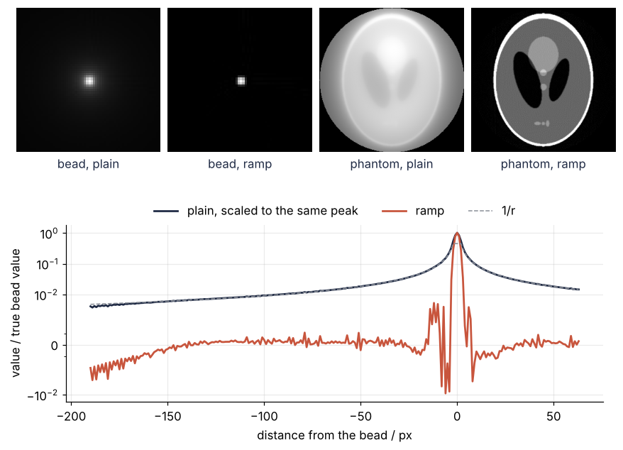
The plain image is in no unit at all: its bead peaks at 5.05, and even after the best scale factor the phantom keeps an RMS error of 0.208. The ramp brings back the slice's own values, the bead as a peak of 1.02 against the true 1 with 99 % of its signal within 3 px, and the phantom with an error of 0.033, six times smaller. The ramp needs no scale factor: scikit-image's ramp is close to \(2|k|\), its sum over angles carries \(\pi/(2N_\theta)\), half the angle step, and the two factors of two cancel.

In the profile the plain curve lies on the dashed \(1/r\) line: \(r\) times its value stays between 4.12 and 4.69 from 10 to 170 px, around the 4.5 of the rings. Beyond 170 px neighboring stripes lie as far apart as the bead is wide, and the halo ripples from angle to angle. The profile runs at 30.5°, halfway between two sampled angles, so that no single stripe dominates it; at the edge, 190 px away, it reads 3.87 between the stripes, where the sampled 30° reads 5.04 on one. The ramp's floor stays within 1.7 % of zero, which the logarithmic axis magnifies into wiggles.

Where it shows up

Medical CT. Filtered back projection with a windowed ramp reconstructed the slices of clinical scanners for decades, and Hounsfield and Cormack shared the 1979 Nobel Prize in Physiology or Medicine for the scanner and its mathematics. A clinical fan beam is not parallel, but its data are rebinned or weighted into the same form and filtered by the same ramp.
Micro-CT of rock cores and fossils. Synchrotron beamlines deliver nearly parallel beams, the geometry of this tutorial. The porosity of a sandstone core and the inner ear of a fossil skull are read off slices reconstructed this way.
Electron tomography of cells and catalyst particles. The specimen holder can tilt only to about ±70°, so a wedge of Fourier space receives no lines at all. The slice theorem says exactly which directions come out blurred.
PET and SPECT. The lines along which a pair of gamma photons or a single photon is detected are projections of the tracer distribution. Clinical scanners reconstruct them mostly iteratively, with OSEM, because they count few photons and the ramp would amplify their noise.
Seismic travel-time tomography. A travel time is the integral of the slowness along a ray, but the rays bend and cover the ground unevenly, so the slice theorem does not hold and the methods are algebraic. The uneven coverage plays the role of the crowded center.
Radio astronomy. Each pair of antennas measures one point of the sky's 2D Fourier transform, and Earth's rotation sweeps it along tracks that crowd the center, which turns a point source into the halo of the "dirty beam". Uniform weighting divides by the sample density, as the ramp does.

Data that sample Fourier space unevenly have to be weighted by the inverse of the sampling density before they are added up, or the dense part dominates the image.

The question

The idea: smear every projection back along its rays

Lines through the center: the Fourier slice theorem

Formalization

See it in code

Where it shows up

Further reading