healpy from the ground up: a CMB sky and the cosmic variance of its spots

The problem: how much can one sky tell you?

The cosmic microwave background fills the sky at 2.7255 K, and on top of that mean it varies by about 100 μK from place to place. Cosmology reads those variations through the angular power spectrum, the variance the sky holds at each angular scale, and healpy is the Python library that pixelizes such a sky, draws it, and measures its spectrum. A map on the sphere is a sum of spherical harmonics, the sphere's version of the sines and cosines of a Fourier series. Each harmonic has a degree ℓ and an order m, and its coefficient is \(a_{\ell m}\). The degree sets the size of a spot, about 180°/ℓ, and \(C_\ell\) is the mean square of the coefficients at fixed ℓ. Planck's first acoustic peak sits near ℓ = 220: spots of about a degree.

The trouble is the count. A degree has only 2ℓ + 1 coefficients on the whole sky, and that is all there is to average over. Even a noiseless, full-sky measurement scatters around the true spectrum by

which is 63 % at the quadrupole ℓ = 2 and 3 % at ℓ = 1000. No better telescope removes that. There is one sky.

So take Planck's best-fit theory spectrum, draw a sky from it, measure the spectrum back, and see what a telescope beam, the pixels, a cut through the galactic plane, and the one-sky limit do to the measurement.

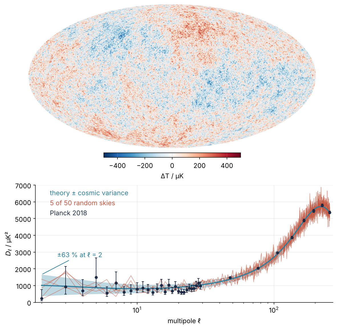
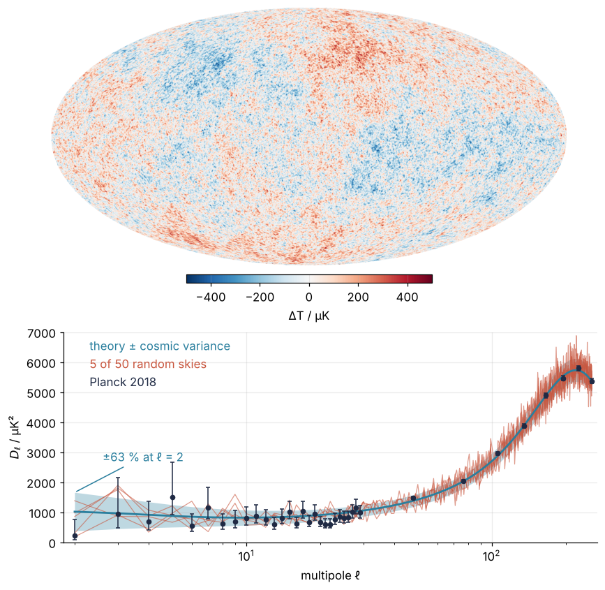
This is where we end up. On top is one sky drawn from the theory. Below it, five of fifty such skies scatter around the theory spectrum as far as cosmic variance says they should, and Planck's measurements of the one real sky scatter the same way. Step 6 draws it.

Setup

The three spectra are Planck's 2018 release (Planck Collaboration, results V and VI, A&A 641, A5 and A6, 2020), fetched from the Planck Legacy Archive's mirror at IRSA: the best-fit theory, 206 kB, and the measured temperature spectrum, unbinned (171 kB) and in bins of Δℓ = 30 (7 kB). Pitfall 2 needs a 14 kB pixel window file from healpy's own data repository. pooch downloads each file once and checks its SHA-256 hash. healpy installs with pip on Linux and macOS, not on Windows; use WSL there.

The files hold \(D_\ell\), a rescaled \(C_\ell\) that Step 3 explains, and healpy wants \(C_\ell\), so the conversion happens on reading. Degrees 0 and 1 stay zero: the monopole is the mean temperature, 2.7255 K, which a map of fluctuations leaves out, and the dipole is dominated by our own motion through the background.

import os
import warnings

warnings.filterwarnings("ignore", message="IProgress not found")  # a tqdm notice at import, not ours
import numpy as np
import matplotlib.pyplot as plt
import healpy as hp
import pooch
from scipy import stats

plt.rcParams.update({
    "figure.figsize": (7, 3.6), "figure.dpi": 110,
    "axes.spines.top": False, "axes.spines.right": False,
    "axes.grid": True, "grid.alpha": 0.25,
    "font.size": 11, "lines.linewidth": 1.8,
})
INK, ACCENT, SECOND, MUTED = "#1f2a44", "#c8553d", "#2a7f9e", "#8a8f98"

NSIDE = 512                  # resolution parameter of the map
LMAX = 2 * NSIDE             # highest degree we synthesize and analyze
FWHM = np.radians(30 / 60)   # a 30 arcmin beam; healpy wants radians
SEED = 2018

pooch.get_logger().setLevel("WARNING")   # no download notice, so a rerun prints the same
CACHE = pooch.os_cache("scistack-healpy")
PLANCK = "https://irsa.ipac.caltech.edu/data/Planck/release_3/ancillary-data/cosmoparams/"
FILES = {
    "theory": ("COM_PowerSpect_CMB-base-plikHM-TTTEEE-lowl-lowE-lensing-minimum-theory_R3.01.txt",
               "50eecd4422e22026070bdacf9fa8a7e7ef3badf4fa50fffea040df669715cf51"),
    "binned": ("COM_PowerSpect_CMB-TT-binned_R3.01.txt",
               "ed2b8b51b033e668e661f6cf4eb7705f15bcaf358189dfc4a4481cc7020130cd"),
    "full": ("COM_PowerSpect_CMB-TT-full_R3.01.txt",
             "ccf3113604020536f6f13ccf51680a7316ad0f32da558eee7f625e613bdd5522"),
}
paths = {key: pooch.retrieve(PLANCK + name, known_hash=f"sha256:{sha}", fname=name, path=CACHE)
         for key, (name, sha) in FILES.items()}
paths["pixwin"] = pooch.retrieve(
    "https://healpy.github.io/healpy-data/pixel_window_functions/pixel_window_n0128.fits",
    known_hash="sha256:830c1edee68c66f3a0545d1bb0202f1740d0eba1ba51bf8c589470029f8079f6",
    fname="pixel_window_n0128.fits",
    path=os.path.join(CACHE, "pixel_window_functions"),   # where hp.pixwin(..., datapath=CACHE) looks
)
for key, p in paths.items():
    print(f"{key:7s} {os.path.getsize(p):8,d} bytes")

theory = np.loadtxt(paths["theory"])     # columns L, TT, TE, EE, BB, PP; D_ell in μK², from ell = 2
binned = np.loadtxt(paths["binned"])     # columns l, Dl, -dDl, +dDl, BestFit; bins of 30 from ell = 30
full = np.loadtxt(paths["full"])         # columns l, Dl, -dDl, +dDl; every ell from 2
ell_th, dl_th = theory[:, 0].astype(int), theory[:, 1]
cl = np.zeros(ell_th[-1] + 1)            # C_ell indexed by ell from 0; monopole and dipole stay zero
cl[ell_th] = 2 * np.pi * dl_th / (ell_th * (ell_th + 1))
print(f"theory: ell = 2 to {ell_th[-1]}, peak D_ell = {dl_th.max():,.0f} μK² at ell = {ell_th[dl_th.argmax()]}")

theory   205,647 bytes
binned     7,143 bytes
full     170,547 bytes
pixwin    14,400 bytes
theory: ell = 2 to 2508, peak D_ell = 5,730 μK² at ell = 220

Step 1: Make a HEALPix map and look at it

HEALPix cuts the sphere into 12 Nside² pixels of equal area, arranged on rings of constant latitude. A map is a plain NumPy array of length npix, and where a pixel sits on the sky follows from its index alone:

for nside in [4, NSIDE]:
    print(f"Nside {nside:3d}: {hp.nside2npix(nside):9,d} pixels, "
          f"{hp.nside2resol(nside, arcmin=True):6.2f} arcmin across, "
          f"{hp.nside2pixarea(nside, degrees=True):8.4f} deg² each")

lon, lat = hp.pix2ang(4, np.arange(6), lonlat=True)
for i in range(6):
    print(f"pixel {i}: longitude {lon[i]:5.1f}°, latitude {lat[i]:4.1f}°")

Nside   4:       192 pixels, 879.48 arcmin across, 214.8592 deg² each
Nside 512: 3,145,728 pixels,   6.87 arcmin across,   0.0131 deg² each
pixel 0: longitude  45.0°, latitude 78.3°
pixel 1: longitude 135.0°, latitude 78.3°
pixel 2: longitude 225.0°, latitude 78.3°
pixel 3: longitude 315.0°, latitude 78.3°
pixel 4: longitude  22.5°, latitude 66.4°
pixel 5: longitude  67.5°, latitude 66.4°

Copy

hp.mollview(np.arange(hp.nside2npix(4)), title="", unit="RING pixel index", cmap="viridis")
hp.graticule(dpar=30, dmer=60, color="white", alpha=0.6)
plt.show()

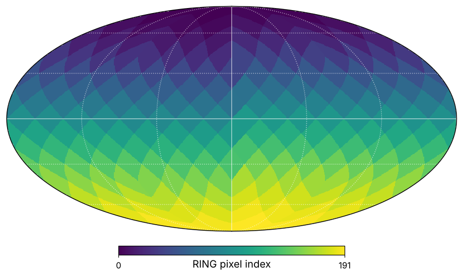
At Nside 512 the map has 3,145,728 pixels, each 6.87 arcmin across and all of the same area. Pixel 0 sits next to the north pole, the first ring holds four pixels at latitude 78.3°, and the index runs ring by ring to the south, as the viridis colors show. This ring order is healpy's default (nest=False); the other order, NESTED, keeps neighbors together for hierarchical work and is not needed here. mollview draws the Mollweide projection, equal-area like the pixels, which is why skies are shown in it (Map projections).

Step 2: Draw a sky from Planck's power spectrum

synfast draws every \(a_{\ell m}\) as a Gaussian number with variance \(C_\ell\) and sums the harmonics on the pixels. It wants \(C_\ell\) from ℓ = 0, which Setup prepared, and it draws from NumPy's global generator, so the seed goes through np.random.seed, not through a default_rng object.

Each degree contributes 2ℓ + 1 modes of variance \(C_\ell\), spread over the 4π of the sphere, so the map's variance should be

np.random.seed(SEED)
m = hp.synfast(cl[:LMAX + 1], NSIDE, lmax=LMAX)

ell = np.arange(LMAX + 1)
rms_pred = np.sqrt(np.sum((2 * ell + 1) * cl[:LMAX + 1]) / (4 * np.pi))
print(f"map RMS {m.std():6.1f} μK   (min {m.min():.0f} μK, max {m.max():.0f} μK)")
print(f"predicted {rms_pred:6.1f} μK")

map RMS  115.2 μK   (min -580 μK, max 552 μK)
predicted  110.2 μK

Copy

hp.mollview(m, title="", unit="ΔT / μK", cmap="RdBu_r", min=-500, max=500)
plt.show()

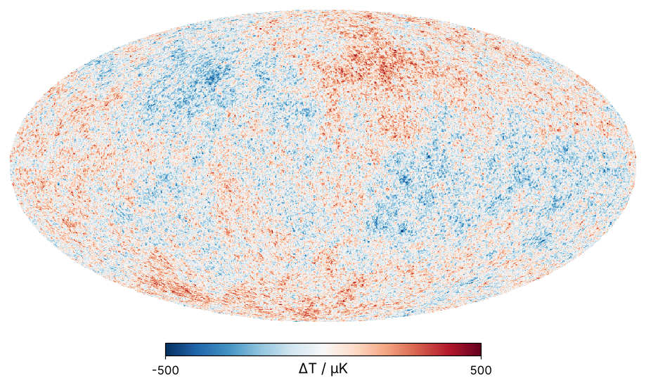
The map's RMS is 115.2 μK against 110.2 μK predicted, 5 μK high, and its extremes are −580 and +552 μK, so the color scale runs to ±500 μK. Spots of about a degree cover the whole sky, as the peak at ℓ = 220 promised, and over them lie a few warm and cool regions tens of degrees across. Both the 5 μK and the large regions belong to this one sky, and Step 3 finds their source.

LMAX is 2 Nside rather than healpy's default of 3 Nside − 1. anafast computes its coefficients as a sum over the pixels, refined by three iterations by default (iter=3), and the result is reliable up to about 2 Nside.

Step 3: Measure the spectrum back with anafast

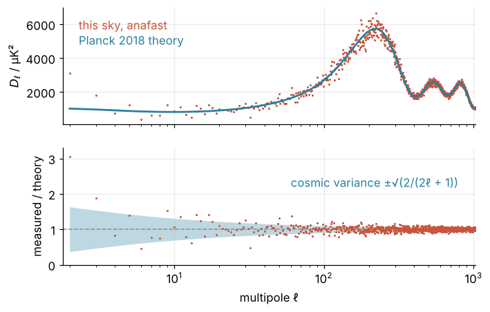
anafast computes the \(a_{\ell m}\) of a map and averages \(|a_{\ell m}|^2\) over the 2ℓ + 1 orders m from −ℓ to ℓ. That average is the estimate \(\hat C_\ell\). A real map ties the negative orders to the positive ones, \(a_{\ell,-m} = (-1)^m a_{\ell m}^*\), so the independent numbers of a degree are the real \(a_{\ell 0}\) and the real and imaginary parts of the ℓ coefficients with m > 0: 2ℓ + 1 real Gaussians, and \(\hat C_\ell/C_\ell\) is the mean of their squares in units of their variance. A squared unit Gaussian has mean 1 and variance 2, so the mean of 2ℓ + 1 of them has mean 1 and variance 2/(2ℓ + 1). That is the √(2/(2ℓ + 1)) of the opening, now with its reason.

The plots use \(D_\ell = \ell(\ell + 1)C_\ell/2\pi\), roughly the variance per logarithmic interval of ℓ, as Planck's files and most papers do: in \(C_\ell\) itself the acoustic peaks vanish under the steep fall. healpy computes in \(C_\ell\), the mean square per mode.

Copy

cl_th = cl[:LMAX + 1]
cl_hat = hp.anafast(m, lmax=LMAX)
to_dl = ell * (ell + 1) / (2 * np.pi)
l2 = ell[2:]                                   # from here on, index 0 is ell = 2
ratio = cl_hat[2:] / cl_th[2:]
cv = np.sqrt(2 / (2 * l2 + 1))

fig, (ax1, ax2) = plt.subplots(2, 1, sharex=True, figsize=(7, 4.4))
ax1.plot(l2, (to_dl * cl_hat)[2:], "o", ms=2, mew=0, color=ACCENT)
ax1.plot(l2, (to_dl * cl_th)[2:], color=SECOND)
ax1.text(2.3, 5700, "this sky, anafast", color=ACCENT)
ax1.text(2.3, 4800, "Planck 2018 theory", color=SECOND)
ax1.set(ylabel=r"$D_\ell$ / μK²", xscale="log")
ax2.fill_between(l2, 1 - cv, 1 + cv, color=SECOND, alpha=0.30, lw=0)
ax2.axhline(1, color=MUTED, ls="--", lw=1)
ax2.plot(l2, ratio, "o", ms=2, mew=0, color=ACCENT)
ax2.text(60, 2.2, "cosmic variance ±√(2/(2ℓ + 1))", color=SECOND)
ax2.set(xlabel="multipole ℓ", ylabel="measured / theory", xlim=(1.8, LMAX), ylim=(0, 3.3))
plt.show()

print(" ell range   mean ratio   scatter   sqrt(2/(2l+1))")
for lo, hi in [(2, 10), (10, 100), (100, 500), (500, LMAX + 1)]:
    s = (l2 >= lo) & (l2 < hi)
    print(f"{lo:4d}-{hi - 1:4d}   {ratio[s].mean():8.3f}   {ratio[s].std():8.3f}   {np.sqrt(np.mean(cv[s]**2)):10.3f}")

excess = 5 * cl_th[2] * (ratio[0] - 1) / (4 * np.pi)
print(f"quadrupole: measured / theory = {ratio[0]:.2f}, adds {excess:,.0f} μK² to the map's variance")
print(f"map variance minus prediction: {m.var() - rms_pred**2:,.0f} μK²")

 ell range   mean ratio   scatter   sqrt(2/(2l+1))
   2-   9      1.332      0.786        0.447
  10-  99      1.008      0.153        0.160
 100- 499      1.001      0.064        0.063
 500-1024      1.002      0.037        0.037
quadrupole: measured / theory = 3.05, adds 867 μK² to the map's variance
map variance minus prediction: 1,120 μK²

Above ℓ = 10 the ratio averages to 1, and its scatter follows the prediction: 0.153 against 0.160 from ℓ = 10 to 99, and 0.037 against 0.037 above ℓ = 500. Below ℓ = 10 one point dominates. This sky's quadrupole is 3.05 times the theory, and its five modes at three times their variance add 867 μK² to the map's variance, most of the 1,120 μK² by which Step 2's map beat the prediction. They are the large warm and cool regions of the map, and Step 6 shows how rare such a sky is.

Step 4: Smooth the sky to a telescope's beam

A telescope sees the sky through a beam. Smoothing is a convolution of the sky with the beam, and on the sphere as on the line a convolution becomes a multiplication of the coefficients (Convolution). A Gaussian beam of full width at half maximum FWHM multiplies every \(a_{\ell m}\) by

so the measured spectrum is \(b_\ell^2 C_\ell\). smoothing applies the beam to a map, gauss_beam returns \(b_\ell\):

m_beam = hp.smoothing(m, fwhm=FWHM, lmax=LMAX)
bl = hp.gauss_beam(FWHM, lmax=LMAX)
cl_beam = hp.anafast(m_beam, lmax=LMAX)

print(" ell    b_l^2   smoothed/theory   divided by b_l^2   unsmoothed/theory")
for l in [100, 220, 400, 500, 600]:
    print(f"{l:4d}   {bl[l]**2:6.3f}   {cl_beam[l] / cl_th[l]:13.3f}   "
          f"{cl_beam[l] / (bl[l]**2 * cl_th[l]):16.4f}   {cl_hat[l] / cl_th[l]:17.4f}")
print(f"b_l^2 falls below 1e-2 at ell = {np.argmax(bl**2 < 1e-2)}")

 ell    b_l^2   smoothed/theory   divided by b_l^2   unsmoothed/theory
 100    0.870           0.903             1.0369              1.0369
 220    0.513           0.493             0.9615              0.9615
 400    0.110           0.102             0.9242              0.9242
 500    0.032           0.032             1.0065              1.0065
 600    0.007           0.007             1.0188              1.0188
b_l^2 falls below 1e-2 at ell = 579

For a close look, gnomview projects a patch onto the plane that touches the sphere at its center, the gnomonic projection, which barely distorts a few degrees. rot=(30, 45) centers it at longitude 30°, latitude 45°, and xsize=400 pixels of reso=3 arcmin make it 20° across, hence the extent. no_plot=True, return_projected_map=True returns the image as an array, so both patches share one figure:

Copy

kw = dict(rot=(30, 45), xsize=400, reso=3, no_plot=True, return_projected_map=True)
patches = [hp.gnomview(x, **kw) for x in (m, m_beam)]
fig, axes = plt.subplots(1, 2, figsize=(7, 3.4), sharey=True, gridspec_kw=dict(wspace=0.15))
for ax, patch, label in zip(axes, patches, ["as drawn", "30 arcmin beam"]):
    im = ax.imshow(patch, origin="lower", cmap="RdBu_r", vmin=-400, vmax=400, extent=(-10, 10, -10, 10))
    ax.text(0, 1.03, label, color=INK, transform=ax.transAxes)
    ax.set(xlabel="x / degrees", xticks=[-10, -5, 0, 5, 10])
    ax.grid(False)
axes[0].set(ylabel="y / degrees")
fig.colorbar(im, ax=axes, label="ΔT / μK", shrink=0.85)
plt.show()

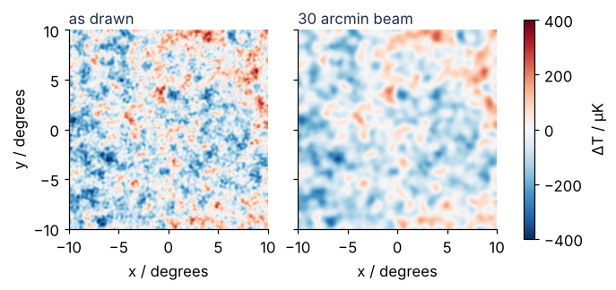
The beam keeps 51 % of the power at ℓ = 220, 3.2 % at ℓ = 500, and under 1 % at ℓ = 600. In the patches the spots blur and the smallest disappear. Divide by \(b_\ell^2\) and the ratio is back at the unsmoothed sky's, to all four digits shown: in a map without noise the beam destroys nothing that the division cannot restore. A real map also carries the detector's noise, which the beam does not smooth, and dividing by a tiny \(b_\ell^2\) multiplies that noise by a huge factor. Divide only where \(b_\ell^2\) stays above about \(10^{-2}\), here up to ℓ = 578.

Step 5: Mask the galactic plane

The Milky Way's own emission covers the galactic plane, and analyses cut it out. Take the map's coordinates as galactic and drop every pixel within 20° of the equator; the sky fraction left, \(f_{\rm sky}\), should be 1 − sin 20°:

npix = hp.nside2npix(NSIDE)
lon, lat = hp.pix2ang(NSIDE, np.arange(npix), lonlat=True)
mask = np.abs(lat) > 20
fsky = mask.mean()
print(f"f_sky = {fsky:.4f}   1 - sin 20° = {1 - np.sin(np.radians(20)):.4f}")

f_sky = 0.6582   1 - sin 20° = 0.6580

Copy

m_shown = hp.ma(m)
m_shown.mask = ~mask                 # a masked array hides where its mask is True
hp.mollview(m_shown, title="", unit="ΔT / μK", cmap="RdBu_r", min=-500, max=500, badcolor=MUTED)
plt.show()

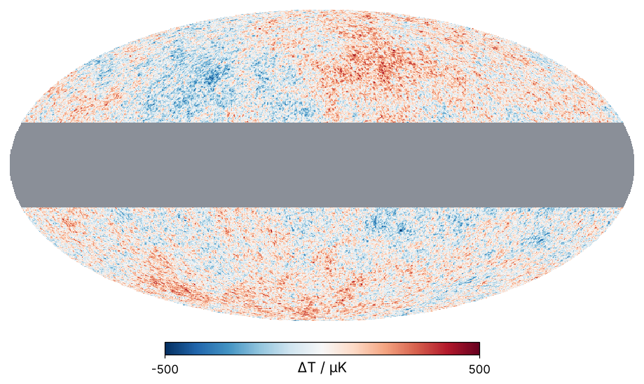
\(f_{\rm sky}\) is 0.6582, against 0.6580 for the exact band. The masked map is zero on a third of the sphere, so its mean square, \(\sum(2\ell + 1)C_\ell/4\pi\) by Step 2, drops to \(f_{\rm sky}\) of the full sky's, and on average every degree loses that share. And multiplying by the mask is, in harmonic coefficients, a convolution with the mask's own coefficients: the smearing that a finite record gives a Fourier spectrum, now in ℓ. The mask's coefficients sit mostly at low degrees, so each degree mixes with neighbors a few degrees away. At ℓ = 500 those neighbors carry nearly the same power and the mixing does not show; at ℓ = 5 they are a large part of the spectrum.

Compare the cut sky with the same sky's full spectrum from Step 3, so that only the mask's effect is left:

cl_cut = hp.anafast(m * mask, lmax=LMAX)

print(" ell range   cut/full   cut/(f_sky full)   scatter")
for lo, hi in [(2, 10), (10, 30), (30, 100), (100, 500), (500, LMAX + 1)]:
    s = slice(lo, hi)
    r = cl_cut[s] / (fsky * cl_hat[s])
    print(f"{lo:4d}-{hi - 1:4d}   {(cl_cut[s] / cl_hat[s]).mean():8.3f}   {r.mean():16.3f}   {r.std():7.3f}")

 ell range   cut/full   cut/(f_sky full)   scatter
   2-   9      0.880              1.337     0.700
  10-  29      0.717              1.089     0.212
  30-  99      0.670              1.017     0.145
 100- 499      0.663              1.008     0.055
 500-1024      0.660              1.003     0.032

Above ℓ = 30 the cut sky keeps 66 % of the power, and dividing by \(f_{\rm sky}\) brings it to within 2 % of the full sky. Below ℓ = 30 the corrected ratio wanders off, to 1.34 for ℓ = 2 to 9 and 1.09 for ℓ = 10 to 29. The spectrum of a cut sky is called the pseudo-\(C_\ell\), and the full correction inverts the mixing with a coupling matrix computed from the mask (Hivon et al. 2002). Above ℓ = 30 the error bars widen, and Step 6 measures by how much.

Step 6: Draw fifty skies and see cosmic variance

One sky is one draw, and a spread shows only over many: fifty skies at Nside 128, each analyzed on the full sky and through the cut of Step 5. A spread estimated from N draws is itself uncertain by a fraction \(1/\sqrt{2(N-1)}\), the standard error of a standard deviation, and a fraction p of N draws by the binomial error \(\sqrt{p(1-p)/N}\). At the quadrupole, \(\hat C_2\) is the mean of five squared Gaussians (Step 3), so \(5\hat C_2/C_2\) follows a χ² distribution with five degrees of freedom, which stats.chi2 evaluates:

NSIDE_E, LMAX_E, N_SKY = 128, 256, 50
ell_e = np.arange(LMAX_E + 1)
cl_e = cl[:LMAX_E + 1]
_, lat_e = hp.pix2ang(NSIDE_E, np.arange(hp.nside2npix(NSIDE_E)), lonlat=True)
mask_e = np.abs(lat_e) > 20
fsky_e = mask_e.mean()

np.random.seed(SEED + 1)
cl_full = np.empty((N_SKY, LMAX_E + 1))
cl_part = np.empty((N_SKY, LMAX_E + 1))
for i in range(N_SKY):
    sky = hp.synfast(cl_e, NSIDE_E, lmax=LMAX_E)
    cl_full[i] = hp.anafast(sky, lmax=LMAX_E)
    cl_part[i] = hp.anafast(sky * mask_e, lmax=LMAX_E)

r_full = cl_full[:, 2:] / cl_e[2:]                 # index 0 is ell = 2
print(" ell   spread of 50 skies   sqrt(2/(2l+1))")
for l in [2, 5, 10, 30, 100, 250]:
    print(f"{l:4d}   {r_full[:, l - 2].std(ddof=1):12.3f}   {np.sqrt(2 / (2 * l + 1)):14.3f}")
print(f"fifty draws fix a spread to about ±{1 / np.sqrt(2 * (N_SKY - 1)):.0%}")
p_low = stats.chi2.cdf(5, 5)
print(f"quadrupole below the theory in {(r_full[:, 0] < 1).mean():.0%} of skies, "
      f"chi-squared with 5 degrees of freedom: {p_low:.0%} ± {np.sqrt(p_low * (1 - p_low) / N_SKY):.0%}")
print(f"skies with a quadrupole as high as Step 2's ({ratio[0]:.2f}): {stats.chi2.sf(5 * ratio[0], 5):.1%}")

 ell   spread of 50 skies   sqrt(2/(2l+1))
   2          0.531            0.632
   5          0.399            0.426
  10          0.275            0.309
  30          0.203            0.181
 100          0.091            0.100
 250          0.061            0.063
fifty draws fix a spread to about ±10%
quadrupole below the theory in 52% of skies, chi-squared with 5 degrees of freedom: 58% ± 7%
skies with a quadrupole as high as Step 2's (3.05): 0.9%

The spread follows √(2/(2ℓ + 1)) to within 12 %, near the ±10 % that fifty draws allow, except at ℓ = 2: 0.53 against 0.63. There the χ² is lopsided, with a long tail to the high side, so a few skies land far above the theory and more land a little below: 58 % by the χ², 52 % of the fifty, inside the ±7 %. Step 2's sky, at 3.05, is a one-in-a-hundred draw.

A cut sky keeps about \(f_{\rm sky}\) of the 2ℓ + 1 modes of each degree, so the relative error of a bin \(b\) of degrees grows to

Average the fifty cut skies in Planck's bins of Δℓ = 30:

r_part = cl_part[:, 2:] / (fsky_e * cl_e[2:])
print(f"f_sky = {fsky_e:.4f}")
print("   bin     mean   spread   full sky   cut sky   spread/cut sky")
for lo in range(30, 240, 30):
    l_bin = np.arange(lo, lo + 30)
    b = r_part[:, l_bin - 2].mean(axis=1)          # the bin average of each sky
    n_modes = np.sum(2 * l_bin + 1)
    print(f"{lo:3d}-{lo + 29:3d}   {b.mean():5.3f}   {b.std(ddof=1):6.3f}   "
          f"{np.sqrt(2 / n_modes):8.3f}   {np.sqrt(2 / (fsky_e * n_modes)):7.3f}   "
          f"{b.std(ddof=1) / np.sqrt(2 / (fsky_e * n_modes)):14.2f}")

q = full[0, 1] / dl_th[0]
print(f"Planck's quadrupole: D_2 = {full[0, 1]:.0f} μK² against {dl_th[0]:.0f} μK² in theory, ratio {q:.2f}")
print(f"skies as low: {(r_full[:, 0] < q).sum()} of {N_SKY}; chi-squared gives {stats.chi2.cdf(5 * q, 5):.1%}")

f_sky = 0.6589
   bin     mean   spread   full sky   cut sky   spread/cut sky
 30- 59   1.026    0.034      0.027     0.034             1.02
 60- 89   1.010    0.027      0.021     0.026             1.04
 90-119   1.001    0.023      0.018     0.022             1.03
120-149   1.004    0.018      0.016     0.019             0.93
150-179   0.999    0.015      0.014     0.018             0.86
180-209   0.996    0.017      0.013     0.016             1.07
210-239   0.997    0.014      0.012     0.015             0.92
Planck's quadrupole: D_2 = 226 μK² against 1017 μK² in theory, ratio 0.22
skies as low: 3 of 50; chi-squared gives 4.7%

In every bin the spread exceeds the full-sky value and lies at 0.86 to 1.07 of the cut-sky formula, as close as fifty draws allow. The rule holds for such bins, not for single degrees, which the mask mixes, nor below ℓ ≈ 30 (Step 5).

Planck's own quadrupole is 0.22 of the theory, below the ±63 % band. Three of the fifty skies went lower, and the χ² gives 4.7 %: one sky in twenty is that quiet, so it is a fact about our sky, not a failure of the model.

Copy

proj = hp.projector.MollweideProj(xsize=1600)     # an array, not mollview's own figure, for the two panels
sky_img = proj.projmap(m, lambda x, y, z: hp.vec2pix(NSIDE, x, y, z))
sky_img = np.ma.masked_invalid(sky_img)            # outside the ellipse

fig = plt.figure(figsize=(8, 7.6))
ax_map = fig.add_axes([0.08, 0.53, 0.84, 0.45])        # the ellipse fills the width
im = ax_map.imshow(sky_img, origin="lower", cmap="RdBu_r", vmin=-500, vmax=500)
ax_map.set_axis_off()
cax = fig.add_axes([0.3, 0.505, 0.4, 0.014])
fig.colorbar(im, cax=cax, orientation="horizontal", label="ΔT / μK")

ax = fig.add_axes([0.1, 0.06, 0.87, 0.36])
dl_e = ell_e * (ell_e + 1) * cl_e / (2 * np.pi)
cv_e = np.sqrt(2 / (2 * ell_e[2:] + 1))
ax.fill_between(ell_e[2:], dl_e[2:] * (1 - cv_e), dl_e[2:] * (1 + cv_e), color=SECOND, alpha=0.30, lw=0)
for i in range(5):
    ax.plot(ell_e[2:], (ell_e * (ell_e + 1) * cl_full[i] / (2 * np.pi))[2:], color=ACCENT, lw=0.8, alpha=0.6)
ax.plot(ell_e[2:], dl_e[2:], color=SECOND, zorder=3)  # the theory on top of the skies
low = full[:28]                                    # ell = 2 to 29, unbinned
ax.errorbar(low[:, 0], low[:, 1], yerr=[low[:, 2], low[:, 3]], fmt="o", ms=4, capsize=2, lw=1, color=INK, zorder=4)
hi = binned[binned[:, 0] < LMAX_E]
ax.errorbar(hi[:, 0], hi[:, 1], yerr=[hi[:, 2], hi[:, 3]], fmt="o", ms=4, capsize=2, lw=1, color=INK, zorder=4)
ax.text(2.3, 6400, "theory ± cosmic variance", color=SECOND)
ax.text(2.3, 5800, "5 of 50 random skies", color=ACCENT)
ax.text(2.3, 5200, "Planck 2018", color=INK)
ax.annotate("±63 % at ℓ = 2", xy=(2, dl_e[2] * 1.63), xytext=(2.6, 2700), color=SECOND,
            arrowprops=dict(arrowstyle="-", color=SECOND, lw=1))
ax.set(xscale="log", xlim=(1.8, 270), ylim=(0, 7000), xlabel="multipole ℓ", ylabel=r"$D_\ell$ / μK²")
plt.show()

Pitfalls

Mixing \(C_\ell\) and \(D_\ell\). Planck's files, and most published plots, hold \(D_\ell\); synfast wants \(C_\ell\), and it accepts either without a word. Feed it the \(D_\ell\) column and the map comes out far too loud and full of pixel-scale grain:

dl_from0 = np.zeros(LMAX_E + 1)
dl_from0[2:] = dl_th[:LMAX_E - 1]
np.random.seed(0)
rms_c = hp.synfast(cl_e, NSIDE_E, lmax=LMAX_E).std()
rms_d = hp.synfast(dl_from0, NSIDE_E, lmax=LMAX_E).std()
print(f"from C_ell: RMS {rms_c:7.1f} μK")
print(f"from D_ell: RMS {rms_d:7.1f} μK, {rms_d / rms_c:.0f} times larger")

from C_ell: RMS    94.8 μK
from D_ell: RMS  4881.1 μK, 51 times larger

The map is 51 times too loud. The \(D_\ell\) column weights each degree by ℓ(ℓ + 1)/2π, over 10,000 at ℓ = 256, so the smallest scales take over the map. Step 3 says why both conventions exist. Convert on reading, compute in \(C_\ell\), plot in \(D_\ell\).

Forgetting the pixel window. A pixel's value is an average over its area, and averaging smooths like a small beam. Degrade the Nside 512 sky to Nside 128 with ud_grade, which averages 16 pixels into one, and compare its spectrum with the one of Step 3:

m_low = hp.ud_grade(m, 128)
cl_low = hp.anafast(m_low, lmax=LMAX_E)
pl = hp.pixwin(128, lmax=LMAX_E, datapath=CACHE)
print(" ell   degraded/original   p_l^2   divided by p_l^2")
for l in [50, 100, 200, 256]:
    print(f"{l:4d}   {cl_low[l] / cl_hat[l]:17.3f}   {pl[l]**2:5.3f}   {cl_low[l] / (pl[l]**2 * cl_hat[l]):16.3f}")

 ell   degraded/original   p_l^2   divided by p_l^2
  50               0.986   0.986              1.001
 100               0.951   0.944              1.008
 200               0.805   0.794              1.014
 256               0.716   0.683              1.048

At ℓ = 200 the degraded map has lost 20 % of its power and at ℓ = 256 already 28 %. The pixel window \(p_\ell^2\) from hp.pixwin accounts for most of it: after the division the ratio is within 1.4 % of 1 up to ℓ = 200, and 4.8 % high at ℓ = 256. datapath points healpy at the file pinned in Setup; without it, healpy downloads its own copy. Divide by \((b_\ell p_\ell)^2\) whenever the map came from real pixels; synfast(..., pixwin=True) applies the same window on the way in.

Giving the beam width in degrees or arcminutes. fwhm in smoothing, synfast, and gauss_beam is in radians, and nothing warns you otherwise:

print(f"fwhm=30:                    RMS {hp.smoothing(m_low, fwhm=30).std():.2e} μK")
print(f"fwhm=np.radians(30 / 60):   RMS {hp.smoothing(m_low, fwhm=FWHM).std():.1f} μK")

fwhm=30:                    RMS 0.00e+00 μK
fwhm=np.radians(30 / 60):   RMS 89.6 μK

fwhm=30 is a beam 30 radians wide, larger than the sphere, which removes every degree above zero and leaves a map with an RMS of exactly zero. Write np.radians(arcmin / 60) every time.

Variations

• Polarization. Pass the TT, EE, BB, and TE columns of the same theory file to synfast(..., new=True) and get maps of I, Q, and U; anafast of the three returns six spectra.
• Instrument noise. Add white noise of σ per pixel. The measured spectrum gains a flat \(N_\ell = \sigma^2 \Omega_{\rm pix}\), with \(\Omega_{\rm pix}\) from hp.nside2pixarea, which must be subtracted before the beam is divided out.
• A mask with soft edges. Smooth the binary mask with hp.smoothing, and divide by the mean of the squared mask instead of \(f_{\rm sky}\); for a smooth mask that mean is no longer the sky fraction.
• Events instead of a field. Arrival directions of gamma-ray photons or neutrinos become a HEALPix count map with hp.ang2pix and np.bincount(..., minlength=npix), and everything from Step 3 on applies.

Cheat sheet

npix, res = hp.nside2npix(nside), hp.nside2resol(nside, arcmin=True)  # 12 Nside² equal-area pixels
lon, lat = hp.pix2ang(nside, np.arange(npix), lonlat=True)     # pixel centers in degrees, RING order
np.random.seed(0); m = hp.synfast(cl, nside, lmax=lmax)         # cl indexed from ell = 0, in C_ell
cl_hat = hp.anafast(m, lmax=lmax)                                # keep lmax at about 2 * nside
dl = ell * (ell + 1) * cl / (2 * np.pi)                          # compute in C_ell, plot in D_ell
m_s = hp.smoothing(m, fwhm=np.radians(arcmin / 60))              # fwhm in radians!
bl, pl = hp.gauss_beam(fwhm, lmax=lmax), hp.pixwin(nside, lmax=lmax, datapath=path)
cl_true = hp.anafast(m * mask, lmax=lmax) / (mask.mean() * bl**2 * pl**2)  # only where bl**2 > 1e-2
err = np.sqrt(2 / ((2 * ell + 1) * fsky))                        # cosmic variance; bin it on a cut sky
hp.mollview(m, title="", unit="μK", cmap="RdBu_r", min=-v, max=v)   # symmetric limits

Further reading

• The healpy documentation, in particular its tutorial, and the HEALPix pages for the pixelization behind it.
• Górski et al. (2005), ApJ 622, 759, for HEALPix itself; Zonca et al. (2019), JOSS 4, 1298, for healpy.
• Planck Collaboration (2020), Planck 2018 results V and VI, A&A 641, A5 and A6, for the spectra; Hivon et al. (2002), ApJ 567, 2, for the coupling matrix of a cut sky.
• Dodelson and Schmidt, Modern Cosmology, 2nd edition, for where the acoustic peaks come from.
• Related tutorials on this site: Spherical harmonics with pyshtools: the shape of Earth's gravity field, The Fourier transform: asking a signal how much of each frequency it contains, Convolution: how a small kernel blurs, sharpens, and finds edges, Map projections: why Greenland looks as large as Africa, and what each keeps, Cosmological distances with quad: why the farthest galaxies look larger, and The standard error of the mean: why four times the data halves the error.
• Download the notebook. It was executed with the library versions in the header.