Phase correlation in scikit-image: undo the drift of a time-lapse

The problem: a time-lapse that drifts

You film a fluorescence culture for 50 minutes, one frame a minute, 256 × 256 pixels at 0.65 µm per pixel. The stage drifts. By the last frame the whole field has moved 3.6 px up and 5.9 px right, 2.4 µm and 3.8 µm, smoothly and by less than a pixel per frame. A cell that sits still appears to travel 4.5 µm, seven pixels, over the movie. Before you measure any motion of the cells, the motion of the stage has to come out: that is image registration.

Phase correlation does it with Fourier transforms. It compares the transforms of two frames frequency by frequency, keeps only the differences in phase, and transforms those back; the shift between the frames shows up as one sharp spike at the place it moved to. We do it once by hand with numpy.fft, then with scikit-image's phase_cross_correlation, move the frames back with scipy.ndimage.shift, and check the result against the drift that went into the data and against the noise measured from the frames themselves, a check you can run on your own data. The same call aligns two satellite scenes of a landslide or two diffraction patterns of a crystal.

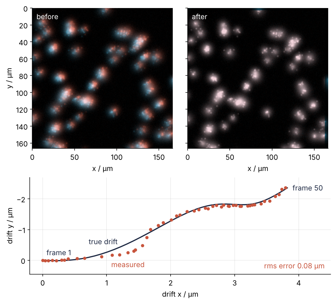
This is where we end up: frame 1 and frame 50 laid on top of each other before and after the correction, and the measured drift of all 50 frames on the drift that was put in. Step 6 draws it. The measured track is off by 0.12 px rms, 0.08 µm, and by 0.45 px at worst.

Setup

The cell below makes frames, an array of shape (50, 256, 256), and keeps the drift it applied as drift, in (row, column) pixels per frame. Frame 1 is frames[0], frame 50 is frames[-1]. The frames are synthetic, so that every number can be checked against the truth: 70 cells built from Gaussian blobs, evaluated at their shifted positions so that each sub-pixel shift is exact, with fresh camera noise in every frame. Random numbers with numpy.random explains the seeded generator, and you can run the cell without reading it. On a real stack, tifffile.imread returns the same kind of array, as Counting cells with scipy.ndimage shows for one frame. estimate_sigma needs PyWavelets: pip install scikit-image PyWavelets.

import numpy as np
import matplotlib.pyplot as plt
import scipy.ndimage as ndi
from skimage.registration import phase_cross_correlation
from skimage.filters import window
from skimage.restoration import estimate_sigma

plt.rcParams.update({
    "figure.figsize": (7, 3.6), "figure.dpi": 110,
    "axes.spines.top": False, "axes.spines.right": False,
    "axes.grid": True, "grid.alpha": 0.25,
    "font.size": 11, "lines.linewidth": 1.8,
})
INK, ACCENT, SECOND, MUTED = "#1f2a44", "#c8553d", "#2a7f9e", "#8a8f98"

N, n_frames = 256, 50          # pixels per side, frames one minute apart
px = 0.65                      # µm per pixel
rng = np.random.default_rng(1)

# 70 cells on a field 15 px wider than the frame on every side, so cells cross the borders
blobs = []                     # (row, column, width / px, brightness) of each Gaussian blob
for _ in range(70):
    cy, cx = rng.uniform(-15, N + 15, 2)
    s = rng.uniform(5, 8)
    blobs.append((cy, cx, s, rng.uniform(0.8, 1.2)))                 # body
    blobs.append((cy, cx, s / 2.5, rng.uniform(0.4, 0.8)))           # nucleus
    for _ in range(rng.integers(3, 7)):                              # granules
        gy, gx = rng.normal(0, 0.6 * s, 2)
        blobs.append((cy + gy, cx + gx, 1.0, rng.uniform(0.4, 0.8)))
cy, cx, width, brightness = np.array(blobs).T

t = np.arange(n_frames)
drift = np.column_stack([-0.08 * t + 0.5 * np.sin(2 * np.pi * t / 35),        # rows, + is down
                         0.12 * t + 0.3 * (1 - np.cos(2 * np.pi * t / 50))])  # columns, + is right

def render(dy, dx):
    # each blob is evaluated at its moved center, so no interpolation enters the data
    r = np.arange(N)
    gy = np.exp(-(r - (cy + dy)[:, None]) ** 2 / (2 * width[:, None] ** 2))
    gx = np.exp(-(r - (cx + dx)[:, None]) ** 2 / (2 * width[:, None] ** 2))
    return 0.1 + (brightness[:, None] * gy).T @ gx

frames = np.array([render(dy, dx) + rng.normal(0, 0.05, (N, N)) for dy, dx in drift])

dy, dx = drift[-1] - drift[0]
print(f"frames {frames.shape}, {px} µm per pixel, field {N * px:.0f} µm wide")
print(f"drift by frame 50 (row, column): ({dy:+.2f}, {dx:+.2f}) px = ({dy * px:+.2f}, {dx * px:+.2f}) µm")

frames (50, 256, 256), 0.65 µm per pixel, field 166 µm wide
drift by frame 50 (row, column): (-3.63, +5.88) px = (-2.36, +3.82) µm

Step 1: Turn a shift into a phase ramp with fft2

np.fft.fft2 is the one-dimensional transform of The Fourier transform applied to every row, then to every column. Each frequency now has two numbers, \(k_y\) waves down the frame and \(k_x\) across it, and one complex value with a magnitude and an angle. Move the image by \(a\) pixels down and \(b\) to the right, and the shift theorem says what happens to its transform:

Every magnitude stays as it was. Every angle changes by an amount that grows in proportion to the frequency: a ramp, whose slope is the shift. To isolate it, take the complex conjugate of \(F_2\), which is the same number with its angle negated. Multiplying \(F_1\) by it multiplies the magnitudes and subtracts the angles. Dividing by the magnitude of the product sets every magnitude to 1 and leaves the angle difference, the ramp alone. This normalized product is called the cross-power spectrum. The division also gives every frequency the same weight, the fine detail of a granule as much as the outline of a whole cell.

F1 = np.fft.fft2(frames[0])
F2 = np.fft.fft2(frames[-1])
R = F1 * np.conj(F2)
R /= np.abs(R)
print(f"|R| from {np.abs(R).min():.3f} to {np.abs(R).max():.3f}")

# the ramp the shift theorem predicts for the true drift, and how far the angle of R strays from it
ky = np.fft.fftfreq(N, 1 / N)[:, None]           # integer frequencies, cycles per frame
kx = np.fft.fftfreq(N, 1 / N)[None, :]
deviation = np.abs(np.angle(R * np.exp(-2j * np.pi * (ky * dy + kx * dx) / N)))
for k in [8, 128]:
    inside = (np.abs(ky) <= k) & (np.abs(kx) <= k)
    print(f"frequencies up to {k:3d}: median deviation from the ramp {np.median(deviation[inside]):.2f} rad")

|R| from 1.000 to 1.000
frequencies up to   8: median deviation from the ramp 0.09 rad
frequencies up to 128: median deviation from the ramp 1.19 rad

Show code

Copy

k = np.fft.fftshift(np.fft.fftfreq(N, 1 / N))
edges = [k[0] - 0.5, k[-1] + 0.5, k[-1] + 0.5, k[0] - 0.5]
fig, ax = plt.subplots(figsize=(4.8, 3.8))
im = ax.imshow(np.angle(np.fft.fftshift(R)), cmap="twilight", vmin=-np.pi, vmax=np.pi, extent=edges)
ax.set(xlim=(-64, 64), ylim=(64, -64),
       xlabel="column frequency / cycles per frame", ylabel="row frequency / cycles per frame")
ax.grid(False)
cb = fig.colorbar(im, ax=ax, ticks=[-np.pi, 0, np.pi])
cb.ax.set_yticklabels(["−π", "0", "π"])
cb.set_label("phase difference / rad")
plt.show()

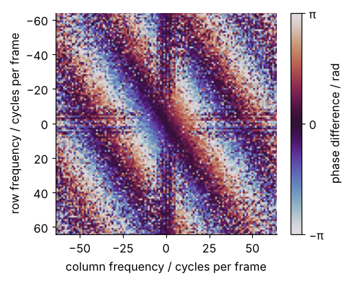
The angle of R, in the cyclic map twilight, is a set of parallel stripes: the ramp, wrapping around every time it climbs by 2π. The stripes run across the direction of the shift and are closer together the larger the shift is. Near the center they are clean, 0.09 rad from the ideal ramp; across all frequencies the median is 1.19 rad, because at the finest frequencies the camera noise outweighs what is left of the cells. The faint cross along the two zero frequencies does not belong to the ramp at all; Pitfall 2 says where it comes from.

Step 2: Turn the ramp into a spike with ifft2

A ramp of angles with all magnitudes 1 is a single wave in two dimensions. A pure tone transforms into one peak at its frequency, and in the same way the inverse transform of a single wave is one spike at one position: the shift. Everywhere else the terms cancel. Step 1 subtracted frame 50's angles from frame 1's, which reverses the ramp, so the spike marks the shift that carries frame 50 back onto frame 1: minus the drift.

corr = np.fft.ifft2(R).real
peak = np.array(np.unravel_index(np.argmax(corr), corr.shape))
print(f"peak at index ({peak[0]}, {peak[1]})")

shift_px = np.where(peak > N // 2, peak - N, peak)    # indices above N/2 are negative shifts
print(f"shift ({shift_px[0]}, {shift_px[1]}) px; true ({-dy:.2f}, {-dx:.2f}) px")
print(f"spike height {corr.max():.3f}, floor scatter {corr.std():.4f}")

peak at index (4, 250)
shift (4, -6) px; true (3.63, -5.88) px
spike height 0.168, floor scatter 0.0039

Index 250 is a shift of -6. The transform treats the frame as a tile repeated in every direction, so positions in its output are counted around a circle from 0 to 255, and a shift of -6 lands at 256 - 6 = 250. Every index above N/2 is a negative shift; MRI k-space reconstruction with numpy.fft shows the same circular order on the frequency side, and fftshift, which the figure uses to put zero in the middle.

Show code

Copy

from matplotlib.patches import Rectangle

c = np.fft.fftshift(corr)
lim = [-N // 2 - 0.5, N // 2 - 0.5, N // 2 - 0.5, -N // 2 - 0.5]
zoom_x = (shift_px[1] - 10.5, shift_px[1] + 10.5)
zoom_y = (shift_px[0] + 10.5, shift_px[0] - 10.5)
fig, (ax1, ax2) = plt.subplots(1, 2, figsize=(7.4, 3.4))
for ax in (ax1, ax2):
    ax.imshow(c, cmap="cividis", extent=lim, vmin=0, vmax=corr.max(), interpolation="nearest")
    ax.grid(False)
    ax.set(xlabel="shift x / px", ylabel="shift y / px")
ax1.add_patch(Rectangle((zoom_x[0], zoom_y[1]), 21, 21, fill=False, ec=MUTED, lw=1.2))   # the zoom
ax2.set(xlim=zoom_x, ylim=zoom_y)
ax2.axvline(-dx, color=MUTED, ls="--", lw=1)
ax2.axhline(-dy, color=MUTED, ls="--", lw=1)
ax2.text(-dx + 0.6, zoom_y[0] - 0.8, "true shift", color=MUTED)
fig.tight_layout()
plt.show()

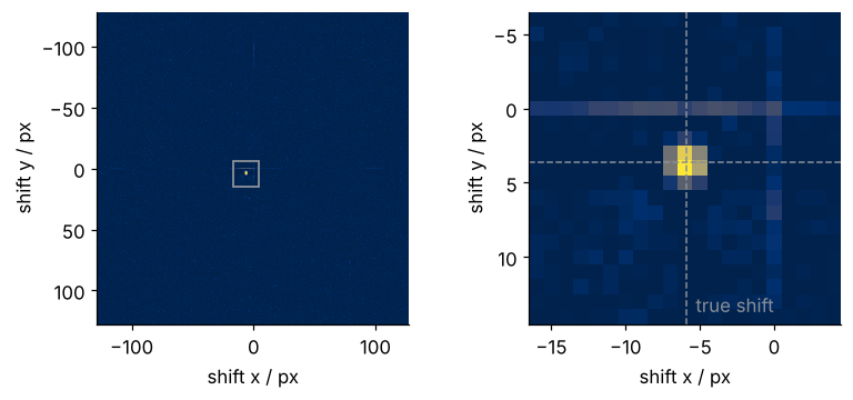
The spike, bright in the sequential map cividis, stands 43 times above the scatter of the floor, and in the zoom it sits on the pixel next to the true shift. The faint lines through zero shift are the cross of Step 1 again. That is the right integer, and no better than an integer.

Step 3: Measure it with phase_cross_correlation

scikit-image does Steps 1 and 2 in one call, with the frame to hold still first and the frame to move second:

shift, error, phasediff = phase_cross_correlation(frames[0], frames[-1])
print(f"shift {shift}, error {error:.4f}, phasediff {phasediff:.3f}")
print("arguments swapped:", phase_cross_correlation(frames[-1], frames[0])[0])

noise = rng.normal(0, 0.05, (N, N))
print(f"error against pure noise: {phase_cross_correlation(frames[0], noise)[1]:.4f}")

shift [ 4. -6.], error 1.0000, phasediff 0.000
arguments swapped: [-4.  6.]
error against pure noise: 1.0000

The shift is (4, -6), as by hand, and three conventions come with it. It is in (row, column) order, rows counted downward. It is the shift that moves the second image onto the first, so it has the sign opposite to the drift. And swapping the arguments flips it. The second return value, error, is 1.0000 here and 1.0000 against a frame of pure noise: with the default normalization="phase" it is not a quality score, and Step 5 gives a check that is. The third, the global phase difference, is zero for real images and is not needed here.

Step 4: Go below a pixel with upsample_factor

The inverse transform of Step 2 is a sum of waves, and a sum can be evaluated at any position, 3.63 as well as 4. That is what upsample_factor does. After finding the integer peak, it evaluates the sum on a grid 1 / upsample_factor px fine, but only in a neighborhood 1.5 px wide around that peak, which is why it is cheap (Guizar-Sicairos and coworkers, 2008, in Further reading).

truth = drift[0] - drift[-1]                 # the shift that moves frame 50 back onto frame 1
for factor in [1, 10, 100, 1000]:
    s = phase_cross_correlation(frames[0], frames[-1], upsample_factor=factor)[0]
    points = int(np.ceil(1.5 * factor)) ** 2 if factor > 1 else 0   # the fine grid around the peak
    print(f"upsample_factor {factor:4d}: shift ({s[0]:6.3f}, {s[1]:6.3f}) px, "
          f"off by {np.hypot(*(s - truth)):.3f} px, {points:9,d} extra points")

upsample_factor    1: shift ( 4.000, -6.000) px, off by 0.392 px,         0 extra points
upsample_factor   10: shift ( 3.600, -5.800) px, off by 0.086 px,       225 extra points
upsample_factor  100: shift ( 3.640, -5.840) px, off by 0.045 px,    22,500 extra points
upsample_factor 1000: shift ( 3.644, -5.840) px, off by 0.046 px, 2,250,000 extra points

The error drops from 0.39 px to 0.09 px at 10 and to 0.045 px at 100, then stops: 1000 evaluates a hundred times as many points and lands within 0.004 px of the answer at 100. The floor is set by the noise and by the frame's edges, which Pitfall 2 takes apart. Use 100.

Step 5: Shift the frame back with ndimage.shift

ndi.shift(frames[-1], shift) moves frame 50 by the shift exactly as phase_cross_correlation returns it. A shift of 3.64 px puts the new pixel centers between the old ones, where the camera measured nothing. The argument order says how a value there is guessed: 0 copies the nearest pixel, which rounds the shift to whole pixels; 1 draws straight lines between neighbors; 3, the default, fits one cubic spline through every pixel of a row and a column and reads it off between them, so even a pixel ten away has a tiny say. The strip the frame moved away from is filled with zeros, so comparisons below leave out a 10 px margin.

Without the truth, check the difference of the two frames: if they are aligned, it is noise only. Each frame carries noise of standard deviation σ, and two independent noises add in variance, σ² + σ², so the difference has a standard deviation of σ√2. estimate_sigma measures σ from each frame through its finest wavelet details, which are noise almost everywhere, and takes their median so that the edges of the cells do not count (Denoise a low-light micrograph with scikit-image explains how).

sigma1, sigma50 = estimate_sigma(frames[0]), estimate_sigma(frames[-1])
floor = np.sqrt(sigma1 ** 2 + sigma50 ** 2)
print(f"noise σ: frame 1 {sigma1:.3f}, frame 50 {sigma50:.3f}, so the floor is {floor:.3f}"
      f"  (top-left corner std {frames[0][:20, :20].std():.3f})")

shift = phase_cross_correlation(frames[0], frames[-1], upsample_factor=100)[0]
aligned = ndi.shift(frames[-1], shift)
inner = (slice(10, -10), slice(10, -10))
rms = lambda a: np.sqrt(np.mean(a[inner] ** 2))
print(f"rms of frame 50 - frame 1: before {rms(frames[-1] - frames[0]):.3f}, "
      f"after {rms(aligned - frames[0]):.3f}, "
      f"with the sign flipped {rms(ndi.shift(frames[-1], -shift) - frames[0]):.3f}")

for order in [0, 3]:
    left = phase_cross_correlation(frames[0], ndi.shift(frames[-1], shift, order=order), upsample_factor=100)[0]
    print(f"order={order}: shift left over after aligning ({left[0]:+.2f}, {left[1]:+.2f}) px")

noise σ: frame 1 0.050, frame 50 0.051, so the floor is 0.072  (top-left corner std 0.145)
rms of frame 50 - frame 1: before 0.408, after 0.066, with the sign flipped 0.624
order=0: shift left over after aligning (-0.21, +0.12) px
order=3: shift left over after aligning (+0.00, +0.00) px

The difference falls from 0.408 to 0.066, just under the floor of 0.072 because the interpolation averages away a little of frame 50's noise. Step 6 adapts this check to a real culture. An empty-looking corner, the estimate Counting cells uses, reports 0.145 here, three times the true noise: the edge of a cell sits in it. With the sign flipped the difference grows to 0.624, worse than not aligning at all. Nearest-neighbor interpolation leaves 0.2 px of shift behind; the cubic default leaves none that registration can find.

Show code

Copy

extent = [10 * px, (N - 10) * px, (N - 10) * px, 10 * px]
fig, axes = plt.subplots(1, 2, figsize=(7.4, 3.5), sharey=True)
for ax, diff, label in zip(axes, [frames[-1] - frames[0], aligned - frames[0]], ["before", "after"]):
    ax.imshow(diff[inner], cmap="gray", vmin=-0.6, vmax=0.6, extent=extent)
    ax.text(0.03, 0.97, label, transform=ax.transAxes, va="top", color="white",
            bbox=dict(facecolor=INK, edgecolor="none", alpha=0.7))
    ax.set(xlabel="x / µm")
    ax.grid(False)
axes[0].set(ylabel="y / µm")
fig.tight_layout()
plt.show()

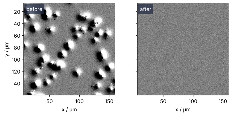
Before alignment every cell appears twice, once bright and once dark; afterwards there is only noise.

Step 6: Track the drift over all 50 frames

Register every frame against frame 1, compare with the truth by the sign rule of Step 3, and move the whole stack back with the shifts found:

measured = np.array([phase_cross_correlation(frames[0], f, upsample_factor=100)[0] for f in frames])
err = measured - (drift[0] - drift)
rms_err = np.sqrt(np.mean(err ** 2, axis=0))
print(f"rms error (row, column): ({rms_err[0]:.3f}, {rms_err[1]:.3f}) px = "
      f"({rms_err[0] * px:.3f}, {rms_err[1] * px:.3f}) µm; largest {np.abs(err).max():.2f} px")
print(f"rms error over both axes: {np.sqrt(np.mean(err ** 2)):.2f} px = {np.sqrt(np.mean(err ** 2)) * px:.2f} µm")

aligned = np.array([ndi.shift(f, s) for f, s in zip(frames, measured)])

# the noise check of Step 5 on neighbors, a minute apart, and on frame 26 aligned one pixel wrong
sigma = np.array([estimate_sigma(f) for f in frames])
floors = np.sqrt(sigma[:-1] ** 2 + sigma[1:] ** 2)
ratio = np.array([rms(b - a) for a, b in zip(aligned[:-1], aligned[1:])]) / floors
wrong = rms(ndi.shift(frames[25], measured[25] + [1, 0]) - aligned[24]) / floors[24]
print(f"aligned neighbors, rms over floor: {ratio.min():.2f} to {ratio.max():.2f}; one pixel wrong: {wrong:.2f}")

rms error (row, column): (0.136, 0.107) px = (0.088, 0.070) µm; largest 0.45 px
rms error over both axes: 0.12 px = 0.08 µm
aligned neighbors, rms over floor: 0.76 to 0.99; one pixel wrong: 1.27

Show code

Copy

from matplotlib.colors import to_rgb

def overlay(a, b):
    # frame a in SECOND, frame b in ACCENT, added on black: where they agree, the sum is near white
    scale = np.percentile(frames[0], 99.5) - 0.1
    norm = lambda f: np.clip((f - 0.1) / scale, 0, 1)[..., None]
    return np.clip(norm(a) * to_rgb(SECOND) + norm(b) * to_rgb(ACCENT), 0, 1)

field = [0, N * px, N * px, 0]
fig = plt.figure(figsize=(7.4, 6.6))
grid = fig.add_gridspec(2, 2, height_ratios=[1.45, 1])
axes = [fig.add_subplot(grid[0, 0]), fig.add_subplot(grid[0, 1])]
for ax, img, label in zip(axes, [overlay(frames[0], frames[-1]), overlay(frames[0], aligned[-1])],
                          ["before", "after"]):
    ax.imshow(img, extent=field)
    ax.text(0.03, 0.97, label, transform=ax.transAxes, va="top", color="white")
    ax.set(xlabel="x / µm")
    ax.grid(False)
axes[0].set(ylabel="y / µm")
axes[1].tick_params(labelleft=False)

ax = fig.add_subplot(grid[1, :])
ax.plot(drift[:, 1] * px, drift[:, 0] * px, color=INK)
ax.plot(-measured[:, 1] * px, -measured[:, 0] * px, "o", color=ACCENT, ms=4)
k = np.argmin(np.abs(drift[:, 1] * px - 1.2))           # name both tracks where they part, near x = 1.2 µm
ax.annotate("true drift", drift[k, ::-1] * px, xytext=(-5, 4), textcoords="offset points",
            color=INK, ha="right")
ax.annotate("measured", -measured[k, ::-1] * px, xytext=(0, -12), textcoords="offset points",
            color=ACCENT, ha="center", va="top")
ax.annotate("frame 1", drift[0, ::-1] * px, xytext=(6, 8), textcoords="offset points", color=INK)
ax.annotate("frame 50", drift[-1, ::-1] * px, xytext=(8, 0), textcoords="offset points",
            color=INK, va="center")
ax.text(0.98, 0.06, f"rms error {np.sqrt(np.mean(err ** 2)) * px:.2f} µm", transform=ax.transAxes,
        ha="right", color=ACCENT)
ax.set(xlabel="drift x / µm", ylabel="drift y / µm", xlim=(-0.2, 4.5), ylim=(0.45, -2.7))
fig.tight_layout()
plt.show()

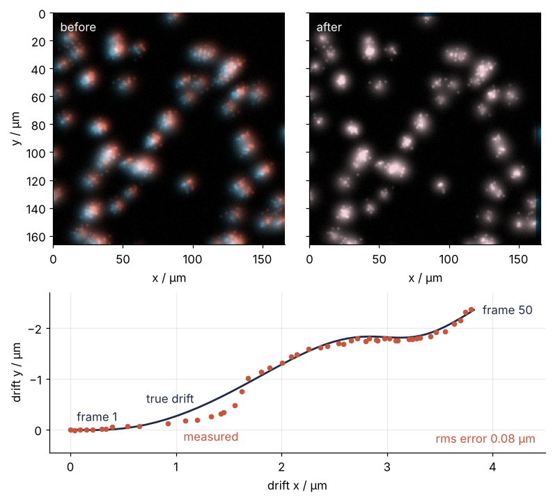
The measured track follows the wobble of the drift, not only its trend, and stays within half a pixel of it in every frame. In the overlay, the teal and red fringes of the uncorrected pair turn into white cells. Every frame is registered against frame 1, not against its neighbor, for the reason in Pitfall 2.

Cells in a real culture move, divide, and bleach, so frame 50 minus frame 1 never reaches the floor. Run Step 5's check on aligned neighbors, a minute apart: here every pair lands between 0.76 and 0.99 of its floor, and a frame aligned one pixel wrong at 1.27. Cell motion lifts every ratio on your own stack; the failed frame is the pair that jumps above the rest. A tenth of a pixel is below what this check sees.

Pitfalls

A rotation is not a shift. Turn frame 50 by a degree before registering it, as a stage that is not quite square does, and the shift comes out wrong:

for angle in [0.5, 1, 2, 5]:
    turned = ndi.rotate(frames[-1], angle, reshape=False)
    s = phase_cross_correlation(frames[0], turned, upsample_factor=100)[0]
    print(f"rotated {angle:3.1f}°: shift ({s[0]:7.2f}, {s[1]:7.2f}) px, off by {np.hypot(*(s - truth)):6.2f} px")

rotated 0.5°: shift (   3.55,   -5.74) px, off by   0.16 px
rotated 1.0°: shift (   2.34,   -6.73) px, off by   1.54 px
rotated 2.0°: shift ( -71.19,   -3.08) px, off by  74.87 px
rotated 5.0°: shift (  -0.04, -121.65) px, off by 115.83 px

At 0.5° the shift is still 0.16 px from the truth, at 1° it is 1.54 px off, and from 2° on it is nonsense. Phase correlation knows translation only: a rotation turns the transform with the image and leaves no single ramp to find. Correct the rotation first, and measure it on the magnitudes of the transforms, which a shift leaves alone (Step 1) and a rotation only turns. skimage.transform.warp_polar resamples them on a grid of angle and radius, where the turn becomes a shift along the angle that phase_cross_correlation measures. scikit-image's gallery example on log-polar registration does this, with both frames faded at the borders as in the next pitfall. Undo the angle with skimage.transform.rotate, then register the shift as in Step 4.

The frame's edges vote for zero. Shifts smaller than a pixel come out too small. The cause is the tile of Step 2: the transform treats the frame as repeated, so the jump from the right border back to the left one, the seam, is a sharp edge. It stays where the frame is and does not move with the stage, so the frequencies it dominates say "shift zero", and the equal weight of Step 1 gives each of them as much say as a frequency carried by the cells. Multiplying both frames by a Hann window, window("hann", shape) from skimage.filters, fades the borders to zero and removes the seam:

hann = window("hann", (N, N))
measured_w = np.array([phase_cross_correlation(frames[0] * hann, f * hann, upsample_factor=100)[0] for f in frames])
rms_w = np.sqrt(np.mean((measured_w - (drift[0] - drift)) ** 2, axis=0))
print(f"rms error over 50 frames (row, column): plain ({rms_err[0]:.3f}, {rms_err[1]:.3f}) px, "
      f"Hann ({rms_w[0]:.3f}, {rms_w[1]:.3f}) px")

true_step = np.mean(drift[:-1, 0] - drift[1:, 0])
for name, w in [("plain", 1), ("Hann", hann)]:
    steps = np.array([phase_cross_correlation(a * w, b * w, upsample_factor=100)[0]
                      for a, b in zip(frames[:-1], frames[1:])])
    end = steps.sum(axis=0) - truth
    print(f"{name:5s}: mean step in rows {steps[:, 0].mean():.3f} px (true {true_step:.3f}), "
          f"steps summed to frame 50 off by ({end[0]:+.2f}, {end[1]:+.2f}) px")

rms error over 50 frames (row, column): plain (0.136, 0.107) px, Hann (0.059, 0.052) px
plain: mean step in rows 0.041 px (true 0.074), steps summed to frame 50 off by (-1.63, +2.32) px
Hann : mean step in rows 0.080 px (true 0.074), steps summed to frame 50 off by (+0.27, -0.27) px

The window more than halves the error of the track. Window your own frames by default; I left it out of Step 6 to keep one idea per step. The price is that cells near the border lose their say, which matters only when what you register on sits there. The bias also explains why Step 6 registers against one reference: between neighboring frames, where the true step is 0.074 px, the plain call measures 0.041, and summed over 49 steps the error reaches 1.6 and 2.3 px at frame 50.

Smoothing first sends the shift to zero. Smooth both frames with ndi.gaussian_filter, as you would before counting cells, and the shift collapses:

for s in [1, 2]:
    smooth = [ndi.gaussian_filter(f, s) for f in (frames[0], frames[-1])]
    found = phase_cross_correlation(*smooth, upsample_factor=100)[0]
    print(f"gaussian_filter sigma={s}: shift ({found[0]:+.2f}, {found[1]:+.2f}) px")
for name, f in [("raw", frames[0]), ("sigma=1", ndi.gaussian_filter(frames[0], 1))]:
    print(f"{name:7s}: mean step between neighbors {np.abs(np.diff(f, axis=1)).mean():.3f}, "
          f"across the seam {np.abs(f[:, 0] - f[:, -1]).mean():.3f}")

gaussian_filter sigma=1: shift (+0.04, -0.03) px
gaussian_filter sigma=2: shift (+0.01, +0.00) px
raw    : mean step between neighbors 0.076, across the seam 0.390
sigma=1: mean step between neighbors 0.036, across the seam 0.385

The smoothing does change the frames: it averages each pixel with its neighbors, which halves the step between them and wipes out the noise and the cells' fine detail. It does not touch the seam, because the last column and the first are neighbors only in the transform's repeated tile, never in the frame gaussian_filter works on, and the step across it goes from 0.390 to 0.385. So the fine frequencies, which carry the step from one pixel to the next and are most of the frequencies, are left with the seam and little else, and they vote for zero as in the previous pitfall. The division of Step 1 then gives them back their full weight. Register the raw frames, and smooth the aligned stack afterwards if counting needs it.

Variations

• A z-stack or a 3D volume. Pass 3D arrays; phase_cross_correlation and ndi.shift take any number of dimensions and return one shift per axis.
• Two satellite scenes. Crop the same area from both and register them. To see whether the shift varies across the scene, register tiles of it: a shift that changes from tile to tile is a warp, not a translation.
• Frames with saturated or dead regions. Pass reference_mask and moving_mask to leave them out; the call then uses masked normalized cross-correlation, and error comes back as NaN.
• A cell's own motion. On the aligned stack, ndi.label and ndi.center_of_mass from Counting cells with scipy.ndimage give the track of a cell, now free of the stage's.

Cheat sheet

from skimage.registration import phase_cross_correlation
shift = phase_cross_correlation(ref, moving, upsample_factor=100)[0]  # raw frames, never smoothed first
# shift is (row, column), rows down; it moves `moving` onto `ref`, opposite to the drift
aligned = ndi.shift(moving, shift)                     # order=3 default; zeros fill the vacated strip
w = skimage.filters.window("hann", ref.shape)          # against the bias of the frame's edges
shift = phase_cross_correlation(ref * w, moving * w, upsample_factor=100)[0]
shifts = [phase_cross_correlation(stack[0], f, upsample_factor=100)[0] for f in stack]  # one reference
floor = np.sqrt(2) * estimate_sigma(ref)               # noise of a difference of two frames
# check rms(aligned[i + 1] - aligned[i]) / floor on neighbors, not against ref: a jump marks a failed frame

Further reading

• The references of skimage.registration.phase_cross_correlation, scipy.ndimage.shift, and skimage.restoration.estimate_sigma.
• scikit-image's gallery examples Image Registration and Using Polar and Log-Polar Transformations for Registration, the second for rotations.
• Guizar-Sicairos, Thurman, Fienup, "Efficient subpixel image registration algorithms", Optics Letters 33, 156 (2008), the upsampling that upsample_factor uses.
• Szeliski, Computer Vision: Algorithms and Applications, 2nd ed. (2022), the chapter on motion estimation.
• Related tutorials on this site: Counting cells with scipy.ndimage: how many are there, and how large?, the prerequisite and what to do with the aligned stack; The Fourier transform: asking a signal how much of each frequency it contains, the other prerequisite; MRI k-space reconstruction with numpy.fft: shifts, fold-over, ringing, the shift theorem from the scanner's side; Denoise a low-light micrograph with scikit-image: what each filter keeps, for estimate_sigma; Fourier fringe analysis and phase unwrapping: a mirror's height map, another measurement read off the phase of a 2D transform.
• Download the notebook. It was executed with the library versions in the header.