Fourier fringe analysis and phase unwrapping: a mirror's height map (Python)

The problem: reading a mirror's surface from its fringes

A Fizeau interferometer tests a polished mirror against a reference flat, here with a He-Ne laser at 632.8 nm. Light reflected from the flat and from the mirror interferes, and tilting the flat a little makes the air gap between them a wedge. The camera then sees straight fringes, each a line of equal gap, one fringe for every λ/2 = 316.4 nm of gap. Where the mirror is higher or lower, the line of equal gap moves sideways, so a bend in a fringe is a height map read in units of 316 nm. Fringe analysis reads those bends to a few nanometers from a single frame, and phase unwrapping is the step where it most often goes wrong.

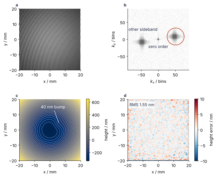
The frame used here has 48 fringes across 40 mm, on a mirror that is a shallow sphere with a 40 nm bump on it. The method is Takeda's: take the 2D Fourier transform of the frame, cut out one of the two copies of the fringe pattern it contains, shift that copy to the center, transform back, take the angle of the complex result, unwrap it, and scale it by λ/4π to get height.

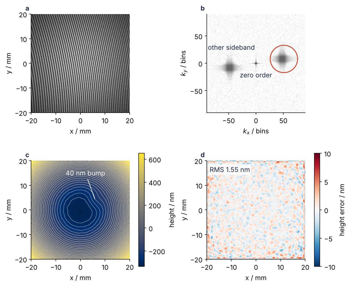
Takeda fringe analysis of a simulated mirror. a: interferogram, 48 tilted fringes. b: its spectrum, with the zero order, the other sideband, and the chosen sideband circled. c: recovered height in nm, a bowl with 25 nm contours that bend around a 40 nm bump. d: error against the true surface, 1.55 nm RMS.

Top left the camera frame, top right its spectrum with the circle the method cuts out, bottom left the height it returns, bottom right that height minus the true surface. The data are simulated from a known surface, so the error can be measured: 1.55 nm RMS over the field, with the largest errors in a thin band along the border. The last step draws this figure.

Setup

Everything under the data generation comment builds the simulated frame: 512 × 512 pixels over 40 × 40 mm, 78 µm per pixel, from the middle of a larger mirror. Its surface rises by 500 nm from the center to x = ±20 mm, and the bump is 40 nm high with a width σ of 2.5 mm, at (6, 4) mm. h_true exists only because the data are simulated, and the steps use it only to measure the error.

Your own frame replaces I: a 2D float array of intensities with straight-looking fringes at least three pixels apart. Turn a frame with nearly horizontal fringes by 90° with np.rot90, because Step 1 looks for the fringe frequency in the right half of the spectrum. Set FOV to the field the frame covers on the mirror and LAM to your laser's wavelength. The grids x, KX, and KY and the matrix A of Step 4 are built from N and assume a square frame, so crop a rectangular one to its central square first, the middle 1024 columns of a 1280 × 1024 camera, and set N = 1024.

import numpy as np
import matplotlib.pyplot as plt
from skimage.restoration import unwrap_phase

N = 512            # pixels per side; the frame must be square
FOV = 40.0         # field of view / mm
dx = FOV / N       # pixel size / mm
LAM = 632.8        # He-Ne wavelength / nm

plt.rcParams.update({
    "figure.figsize": (7, 3.6), "figure.dpi": 110,
    "axes.spines.top": False, "axes.spines.right": False,
    "axes.grid": True, "grid.alpha": 0.25,
    "font.size": 11, "lines.linewidth": 1.8,
})
INK, ACCENT, SECOND, MUTED = "#1f2a44", "#c8553d", "#2a7f9e", "#8a8f98"

x = (np.arange(N) - N // 2) * dx                   # pixel positions / mm, same for y
X, Y = np.meshgrid(x, x)

# ---- data generation: a simulated mirror, not part of the method
h_true = 500 * (X**2 + Y**2) / 20**2 + 40 * np.exp(-((X - 6)**2 + (Y - 4)**2) / (2 * 2.5**2))   # nm
envelope = np.exp(-(X**2 + Y**2) / (2 * 20**2))     # Gaussian illumination, sigma 20 mm

def interferogram(kx, ky, rng):
    """Camera frame with kx and ky fringes across it, contrast 0.7, noise 0.1."""
    n = np.arange(N)
    # an integer number of fringes keeps the carrier periodic across the frame
    carrier = 2 * np.pi * (kx * n[None, :] + ky * n[:, None]) / N
    fringes = envelope * (1 + 0.7 * np.cos(carrier + 4 * np.pi * h_true / LAM))
    return fringes + 0.1 * rng.standard_normal((N, N))

rng = np.random.default_rng(7)
# ---- data: replace I with your own frame
I = interferogram(48, 8, rng)

print(I.shape, f"intensity {I.min():.2f} to {I.max():.2f}, a fringe every {N / np.hypot(48, 8):.1f} pixels")

(512, 512) intensity -0.17 to 1.97, a fringe every 10.5 pixels

Step 1: Find the carrier in the 2D spectrum

Write a pixel's brightness as a mean level \(a\), a fringe contrast \(b\), and a cosine whose phase grows linearly across the frame plus the part you are after, \(\varphi\). A cosine is two complex exponentials, so

\[I(\mathbf x) = a + b\cos(2\pi\,\mathbf f_0\cdot\mathbf x + \varphi) = a + c\,e^{2\pi i\,\mathbf f_0\cdot\mathbf x} + c^*e^{-2\pi i\,\mathbf f_0\cdot\mathbf x}, \qquad c = \tfrac{b}{2}\,e^{i\varphi} .\]

The carrier \(\mathbf f_0\) is the fringe frequency set by the tilt of the reference, here 48 cycles across the frame in \(x\) and 8 in \(y\). The zero order is the peak at zero frequency, the transform of \(a\), which varies only as slowly as the illumination. The sidebands are the two copies of \(c\) around \(+\mathbf f_0\) and \(-\mathbf f_0\), named after those of an AM radio signal. Either one carries \(\varphi\).

They are not points. Where \(\varphi\) changes, the fringes are locally denser or sparser, and the local fringe frequency differs from \(\mathbf f_0\) by \(|\nabla\varphi|/2\pi\). Each sideband is a lobe whose half-width is the largest of these differences, and the method works while the lobe stays clear of the zero order. The simulation knows \(\varphi = 4\pi h/\lambda\), so the half-width can be computed:

gy, gx = np.gradient(4 * np.pi * h_true / LAM, dx)      # phase slope / (rad/mm)
half_width = np.hypot(gx, gy).max() / (2 * np.pi) * FOV  # cycles per frame, which are bins
print(f"lobe half-width {half_width:.1f} bins, carrier {np.hypot(48, 8):.1f} bins from the center")

lobe half-width 8.9 bins, carrier 48.7 bins from the center

The steepest slope, at the corners, gives 8.9 bins, against a carrier 48.7 bins out: plenty of room. Cycles per mm times the 40 mm field are cycles per frame, the unit of one FFT bin. Now the spectrum, centered with fftshift as in MRI k-space reconstruction. The sidebands mirror each other, so the peak search looks in the right half only, outside the 4 bins where the zero order outshines them.

F = np.fft.fftshift(np.fft.fft2(I))
k = np.arange(N) - N // 2                          # bin index, zero in the middle
KX, KY = np.meshgrid(k, k)

def find_peak(F):
    search = (KX > 0) & (np.hypot(KX, KY) > 4)     # right half, outside the zero order
    iy, ix = np.unravel_index(np.where(search, np.abs(F), 0).argmax(), F.shape)
    return KX[iy, ix], KY[iy, ix]

kx0, ky0 = find_peak(F)
print(f"sideband peak at ({kx0}, {ky0}) bins, carrier at (48, 8)")

log_F = np.log10(np.abs(F))
spectrum = dict(cmap="gray_r", vmin=np.median(log_F), origin="lower", extent=[-N / 2 - 0.5, N / 2 - 0.5] * 2)
fig, ax = plt.subplots(figsize=(7, 3.8))
ax.imshow(log_F, **spectrum)                       # dark is strong; the noise floor is white
ax.plot(kx0, ky0, "o", color=ACCENT, ms=4)
phi_circle = np.linspace(0, 2 * np.pi, 200)
ax.plot(kx0 + half_width * np.cos(phi_circle), ky0 + half_width * np.sin(phi_circle), color=SECOND, lw=1.2, ls="--")
ax.set(xlabel="$k_x$ / bins", ylabel="$k_y$ / bins", xlim=(-128, 128), ylim=(-64, 64))
ax.grid(False)
plt.show()

sideband peak at (51, 8) bins, carrier at (48, 8)

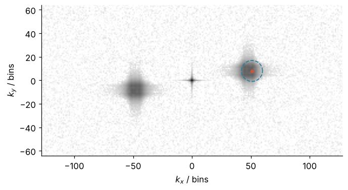
Log magnitude of the interferogram's 2D spectrum in bins, dark where strong. A sharp zero order at the center and two sideband lobes about 49 bins away on either side; a dashed teal circle of 8.9 bins radius marks the lobe around the detected peak on the right.

The peak sits at (51, 8), three bins from the carrier. The lobe's top is nearly flat, so with noise on it the highest bin can land a few bins from its middle.

Step 2: Cut out one sideband and shift it to the center

Keep a disc of radius \(r\) around the peak, set everything else to zero, and roll the disc to the center. The shift is by the detected peak, because on your own frame that is all you have. By the shift theorem from the MRI tutorial's Step 3, moving the spectrum by \(-\mathbf k\), toward the center, multiplies the image by \(e^{-2\pi i\,\mathbf k\cdot\mathbf x}\), so what comes back from ifft2 is \(c\) times \(e^{2\pi i(\mathbf f_0-\mathbf k)\cdot\mathbf x}\). The peak sits three bins right of the carrier, so that leftover factor is a phase falling by three turns across the frame: three fringes of tilt, 3 × 316.4 nm = 949 nm. Step 4 removes it with the mirror's own tilt.

For \(r\), start at half the peak's distance from the center, 25 bins here: wide enough for the 8.9-bin half-width and clear of the zero order. Step 5 tests the choice.

r = int(np.hypot(kx0, ky0) / 2)
window = np.hypot(KX - kx0, KY - ky0) <= r
c = np.fft.ifft2(np.fft.ifftshift(np.roll(F * window, (-ky0, -kx0), axis=(0, 1))))
phase = np.angle(c)
print(f"window radius {r} bins, peak minus carrier ({kx0 - 48}, {ky0 - 8}) bins")
print(f"phase from {phase.min():.4f} to {phase.max():.4f} rad")

extent = [x[0] - dx / 2, x[-1] + dx / 2] * 2
fig, ax = plt.subplots(figsize=(5, 4))
im = ax.imshow(phase, cmap="twilight", vmin=-np.pi, vmax=np.pi, origin="lower", extent=extent)
fig.colorbar(im, ax=ax, label="wrapped phase / rad")
ax.set(xlabel="x / mm", ylabel="y / mm", xlim=(-20, 20), ylim=(-20, 20))
ax.grid(False)
plt.show()

window radius 25 bins, peak minus carrier (3, 0) bins
phase from -3.1416 to 3.1416 rad

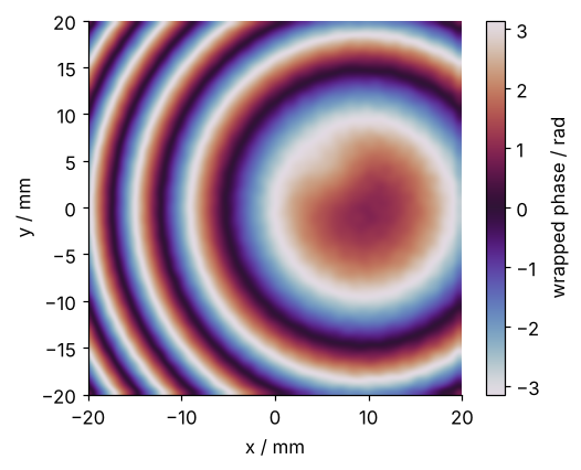
Wrapped phase after the sideband filter, from -π to π in a cyclic color map, x and y in mm over the 40 by 40 mm field. Closed sawtooth rings centered about 10 mm right of the middle, shifted there by the leftover tilt; each jump from π to -π is one wrap.

The window kept \(c\) and nothing of \(a\) or of the other sideband, so the angle of the result is \(\varphi\) plus the three-fringe plane, wrapped into the interval from −π to π. The sawtooth rings are the sphere, centered about 10 mm right of the middle because the plane adds its slope to the sphere's. The bump hides in them.

Step 3: Unwrap the phase, one row and then the whole map

The rule for unwrapping is one sentence: wherever two neighbors differ by more than π, add or subtract 2π from everything after. That is np.unwrap, here on the center row:

row = phase[N // 2]
row_unwrapped = np.unwrap(row)
print(f"jumps larger than π along the row: {np.sum(np.abs(np.diff(row)) > np.pi)}, "
      f"unwrapped span {np.ptp(row_unwrapped):.1f} rad")

fig, ax = plt.subplots()
ax.plot(x, row, color=INK, lw=1.2)
ax.plot(x, row_unwrapped, color=ACCENT)
ax.text(4, 4.5, "wrapped", color=INK)
ax.text(-10, -21, "unwrapped", color=ACCENT)
ax.set(xlabel="x / mm", ylabel="phase / rad", xlim=(-20, 20), ylim=(-26, 7))
plt.show()

jumps larger than π along the row: 5, unwrapped span 21.4 rad

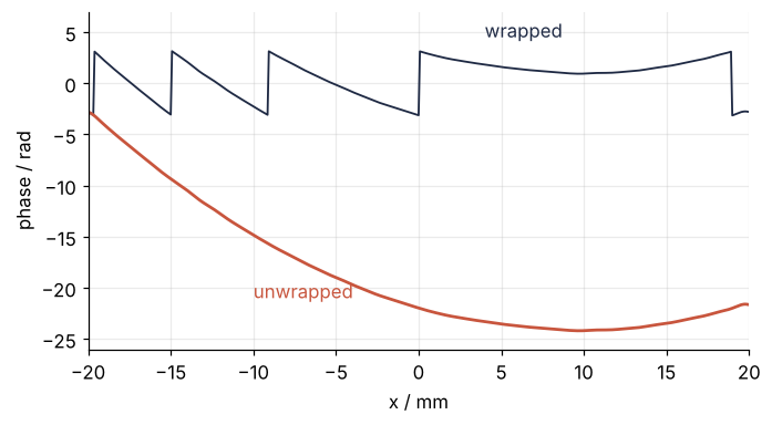
Phase along the center row in radians against x in mm. The wrapped curve jumps by 2π five times; the unwrapped curve is one smooth tilted parabola through them.

Five jumps, and 21.4 rad of smooth phase behind them. In one dimension there is one path from the first pixel to the last, so a single wrong decision, a noisy pixel that looks like a jump, shifts the rest of the row by 2π. In two dimensions every pixel can be reached along many paths, and noise can make them disagree. skimage.restoration.unwrap_phase (Herráez and coworkers, 2002) scores each pixel by how smoothly the wrapped phase runs through it and its neighbors and unwraps the most reliable ones first. The paths between good pixels then run around the noisy ones, so a wrong jump at a noisy pixel stays there:

unwrapped = unwrap_phase(phase, rng=0)             # it draws random numbers inside; seed them
span = unwrapped.max() - unwrapped.min()
print(f"unwrapped map spans {span:.1f} rad, {span / (2 * np.pi):.1f} fringes")

unwrapped map spans 31.2 rad, 5.0 fringes

Almost five fringes, sphere and leftover tilt together, defined only up to a constant multiple of 2π that Step 4 takes care of. Pitfall 2 shows what happens without the ordering.

Step 4: Convert phase to height and remove piston and tilt

The light goes to the mirror and back, so one turn of phase is half a wavelength of height, \(h = \varphi\lambda/4\pi\). Two parts of that height belong to the setup, not to the mirror. Piston is a constant offset, the mean distance between mirror and reference, which one frame cannot measure, and it also absorbs the 2π multiple from Step 3. Tilt is a plane, set by how the mirror sits in its mount and, here, by the three-bin offset from Step 2.

A plane is \(c_0 + c_1 x + c_2 y\), a straight-line fit with one more variable. Stack one row \([1, x, y]\) per pixel into a matrix \(A\), one column per term of the plane. \(A\mathbf c \approx \mathbf h\) is an overdetermined linear system, and np.linalg.lstsq returns its least-squares solution, the same call that fits a line with columns \([1, x]\). The true surface gets the same fit, so that the comparison ignores piston and tilt.

h = unwrapped * LAM / (4 * np.pi)                  # nm
A = np.column_stack([np.ones(N * N), X.ravel(), Y.ravel()])
print("A:", A.shape)

def detilt(h):
    """Subtract the least-squares plane; return the rest and the plane's coefficients."""
    coef, *_ = np.linalg.lstsq(A, h.ravel(), rcond=None)
    return h - (A @ coef).reshape(h.shape), coef

height, coef = detilt(h)
truth, _ = detilt(h_true)
error = height - truth
print(f"fitted tilt across the frame: {coef[1] * FOV:.0f} nm in x, {coef[2] * FOV:.0f} nm in y")

border = round(1 / dx)                             # 1 mm in pixels
inner = error[border:-border, border:-border]
near_bump = np.hypot(X - 6, Y - 4) < 5             # within 2 sigma of the bump
print(f"RMS error {np.sqrt(np.mean(error**2)):.2f} nm, largest {np.abs(error).max():.1f} nm")
print(f"RMS error without a 1 mm border {np.sqrt(np.mean(inner**2)):.2f} nm")
print(f"largest error within 5 mm of the 40 nm bump {np.abs(error[near_bump]).max():.2f} nm")

A: (262144, 3)
fitted tilt across the frame: -951 nm in x, -3 nm in y
RMS error 1.55 nm, largest 15.1 nm
RMS error without a 1 mm border 1.26 nm
largest error within 5 mm of the 40 nm bump 3.04 nm

The fitted tilt is −951 nm in \(x\) against the 949 nm predicted from the three-bin offset, and nearly nothing in \(y\), where the peak sat on the carrier. The recovered height is off by 1.55 nm RMS and by 15.1 nm at worst. Without a 1 mm border the RMS drops to 1.26 nm: the worst errors sit in a thin band at the edges, where the FFT treats the frame as periodic and the sphere's slope jumps from +50 to −50 nm per mm across the seam. Within 5 mm of the bump's center the error is at most 3.04 nm, against a height of 40 nm.

Step 5: Choose the window size, and draw the result

Wrap Steps 1 to 4 in one function and sweep the window radius. Here the truth says which radius is best:

def height_from(I, r):
    F = np.fft.fftshift(np.fft.fft2(I))
    kx0, ky0 = find_peak(F)
    window = np.hypot(KX - kx0, KY - ky0) <= r
    c = np.fft.ifft2(np.fft.ifftshift(np.roll(F * window, (-ky0, -kx0), axis=(0, 1))))
    return detilt(unwrap_phase(np.angle(c), rng=0) * LAM / (4 * np.pi))[0]

print("r / bins   RMS error / nm   without the 1 mm border / nm")
for r_try in [6, 10, 12, 14, 18, 25, 32, 48]:
    err = height_from(I, r_try) - truth
    err_inner = err[border:-border, border:-border]
    print(f"{r_try:8d}   {np.sqrt(np.mean(err**2)):14.2f}   {np.sqrt(np.mean(err_inner**2)):29.2f}")

r / bins   RMS error / nm   without the 1 mm border / nm
       6           118.94                           93.12
      10             6.45                            4.47
      12             3.68                            2.24
      14             2.49                            1.38
      18             1.77                            1.09
      25             1.55                            1.26
      32             1.76                            1.59
      48             2.59                            2.42

Below the lobe's 8.9-bin half-width the window cuts off the steepest parts of the sphere: 119 nm at 6 bins. Centered on the peak, three bins off the carrier, the window holds the whole lobe only from about 12 bins on, where the full RMS is down to 3.68 nm. Past that, the error inside the border is lowest at 18 bins, 1.09 nm, and grows with every wider window, which adds noise. The full RMS keeps falling to 1.55 nm at 25 bins, because the slope jump at the frame's edges is sharp, and a wider window keeps more of its broad spectrum.

On your own frame there is no h_true, so set \(r\) to half the peak's distance from the center and check on the spectrum that the lobe fits inside that circle; if it does not, the carrier is too low (Pitfall 1). Here the rule gives 25 bins, the best error over the whole map, the number you report. If you discard the border anyway, twice the lobe's half-width, 18 bins here, does 0.17 nm better inside it. The figure from the motivation:

height = height_from(I, r)
error = height - truth
rms = np.sqrt(np.mean(error**2))

fig, axes = plt.subplots(2, 2, figsize=(8, 6.8), layout="constrained")
(ax_i, ax_f), (ax_h, ax_e) = axes
ax_i.imshow(I, cmap="gray", origin="lower", extent=extent)
ax_f.imshow(log_F, **spectrum)
ax_f.plot(kx0 + r * np.cos(phi_circle), ky0 + r * np.sin(phi_circle), color=ACCENT, lw=1.6)
ax_f.text(0, -14, "zero order", color=INK, ha="center", va="top")
ax_f.text(-kx0 + 6, -ky0 + 30, "other sideband", color=INK, ha="center", va="bottom")
ax_f.set(xlim=(-90, 90), ylim=(-90, 90), xlabel="$k_x$ / bins", ylabel="$k_y$ / bins")
im_h = ax_h.imshow(height, cmap="cividis", origin="lower", extent=extent)
ax_h.contour(x, x, height, levels=np.arange(-300, 700, 25), colors="white",
           linewidths=0.6, linestyles="solid", alpha=0.6)                     # 25 nm apart
ax_h.annotate("40 nm bump", (6, 4), xytext=(2, 14), color="white", ha="center",
              arrowprops=dict(arrowstyle="-", color="white", lw=1))
fig.colorbar(im_h, ax=ax_h, label="height / nm", shrink=0.85)
im_e = ax_e.imshow(error, cmap="RdBu_r", vmin=-10, vmax=10, origin="lower", extent=extent)
fig.colorbar(im_e, ax=ax_e, label="height error / nm", shrink=0.85, ticks=[-10, -5, 0, 5, 10])
ax_e.text(0.03, 0.95, f"RMS {rms:.2f} nm", transform=ax_e.transAxes, va="top", color=INK,
          bbox=dict(facecolor="white", edgecolor="none", alpha=0.8, pad=2))
for ax, label in zip(axes.flat, "abcd"):
    ax.text(-0.02, 1.02, label, transform=ax.transAxes, ha="right", va="bottom", color=INK, weight="bold")
    ax.grid(False)
    if ax is not ax_f:
        ax.set(xlabel="x / mm", ylabel="y / mm", xlim=(-20, 20), ylim=(-20, 20))
plt.show()

Takeda fringe analysis of a simulated mirror. a: interferogram, 48 tilted fringes. b: its spectrum, with the zero order, the other sideband, and the chosen sideband circled. c: recovered height in nm, a bowl with 25 nm contours that bend around a 40 nm bump. d: error against the true surface, 1.55 nm RMS.

On a real instrument, the reference flat's own errors and air turbulence add to what the simulation shows.

Pitfalls

A carrier too low. The symptom is a height map off by a hundred nanometers or more, in broad swells that no window size removes. Tilt the reference less, so that only 10 fringes cross the frame, and the 8.9-bin lobe reaches from about 1 to 19 bins and overlaps the zero order. No window helps then: the rule's window cuts the lobe in half, and one wide enough for the lobe takes in the zero order.

I_low = interferogram(10, 0, np.random.default_rng(7))      # same noise, 10 fringes
kx_low, ky_low = find_peak(np.fft.fftshift(np.fft.fft2(I_low)))
print(f"sideband peak at ({kx_low}, {ky_low}) bins")
for r_try in [int(np.hypot(kx_low, ky_low) / 2), 14]:
    err = height_from(I_low, r_try) - truth
    print(f"r = {r_try:2d} bins   RMS error {np.sqrt(np.mean(err**2)):6.1f} nm")

sideband peak at (13, 0) bins
r =  6 bins   RMS error  119.1 nm
r = 14 bins   RMS error  210.1 nm

119 nm with the rule's 6 bins, 210 nm with 14, against 1.55 nm at 48 fringes. The fix is in the instrument: tilt the reference for more fringes, so the carrier sits at least twice the lobe's half-width from the center with room for the zero order, but keep three or more pixels per fringe.

Unwrapping through bad pixels. The symptom is a streak that runs from a bad spot to the edge of the frame, offset by a multiple of 316 nm. A dust speck or a saturated patch gives a few pixels of random phase, and unwrapping row by row, then column by column, carries each wrong jump along the rest of its path. Here an 8 × 8 patch of random phase goes into the wrapped map from Step 2:

bad = phase.copy()
bad[300:308, 200:208] = rng.uniform(-np.pi, np.pi, (8, 8))

def wrong_pixels(result):
    """Phase error against the clean unwrapped map, with the overall 2π multiple removed."""
    diff = result - unwrapped
    return diff - 2 * np.pi * np.round(np.median(diff) / (2 * np.pi))

err_rows = wrong_pixels(np.unwrap(np.unwrap(bad, axis=1), axis=0))
err_skimage = wrong_pixels(unwrap_phase(bad, rng=0))
print(f"pixels off by more than π: rows then columns {np.sum(np.abs(err_rows) > np.pi)}, "
      f"unwrap_phase {np.sum(np.abs(err_skimage) > np.pi)}")

fig, axes = plt.subplots(1, 2, figsize=(8, 4), sharey=True, layout="constrained")
for ax, err, name in zip(axes, [err_rows, err_skimage], ["rows, then columns", "unwrap_phase"]):
    im = ax.imshow(err * LAM / (4 * np.pi), cmap="RdBu_r", vmin=-400, vmax=400, origin="lower", extent=extent,
                   interpolation="nearest")
    ax.add_patch(plt.Rectangle((x[200] - 0.5, x[300] - 0.5), 8 * dx + 1, 8 * dx + 1,   # the patch, 0.5 mm around
                               fill=False, ec=MUTED, lw=1, ls="--"))
    ax.text(0.04, 0.04, name, transform=ax.transAxes, color=INK)
    ax.set(xlabel="x / mm", xlim=(-12, 4), ylim=(0, 20), yticks=[0, 5, 10, 15, 20])          # zoom on the patch and the frame's top edge
    ax.grid(False)
axes[0].set(ylabel="y / mm")
fig.colorbar(im, ax=axes, label="height error / nm", shrink=0.85)
plt.show()

pixels off by more than π: rows then columns 834, unwrap_phase 15

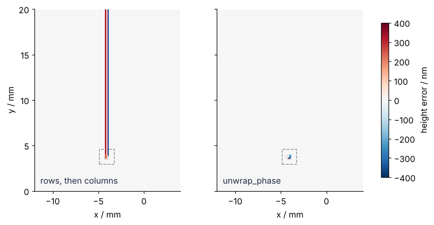
Height error in nm near an 8 by 8 pixel patch of random phase, marked by a dashed square, x and y in mm. Left, rows then columns: a streak of ±316 nm errors runs from the patch to the top edge of the frame. Right, unwrap_phase: the error stays inside the square.

834 pixels go wrong with rows then columns, 15 with unwrap_phase, all of them inside the 64-pixel patch, whose phase was random anyway. When you know where the bad pixels are, do better still and pass them as a mask: np.ma.masked_array(phase, mask) is NumPy's array with a boolean "ignore these" layer, and unwrap_phase leaves masked pixels out of the unwrapping and out of the decisions about their neighbors.

The wrong sideband. The symptom is a map that looks right but upside down: the bump a dent, the bowl a dome. The two sidebands carry \(+\varphi\) and \(-\varphi\), and which one belongs to "+" depends on the direction of the tilt and on the orientation of the camera. Taking the left sideband of this frame returns \(-h\). Check the sign once on the instrument with a known feature, a gentle press on the reference or a part known to be convex, and keep the convention from then on.

Variations

A round mirror. Fill the pixels outside the aperture with the mean intensity before the FFT, and pass the outside as the mask to unwrap_phase, as in Pitfall 2.
Phase shifting instead of a carrier. With a piezo moving the reference, four frames shifted by π/2 each give \(\varphi = \operatorname{atan2}(I_4 - I_2,\, I_1 - I_3)\) per pixel, with no window and full resolution. Unwrapping stays the same.
Satellite radar (InSAR). The interferogram arrives as complex numbers with the phase already in them, and the 2D unwrapping is the same problem on noisier data, with water and layover (steep slopes that the radar images folded over) masked out.
Name the aberrations. Fit the height map with Zernike polynomials, the same lstsq call with more columns. The sphere comes out as defocus.

Cheat sheet

F = np.fft.fftshift(np.fft.fft2(I))                          # zero frequency in the middle
search = (KX > 0) & (np.hypot(KX, KY) > 4)                    # right half, outside the zero order
iy, ix = np.unravel_index(np.argmax(np.where(search, abs(F), 0)), F.shape)
kx0, ky0 = KX[iy, ix], KY[iy, ix]                            # sideband peak / bins
window = np.hypot(KX - kx0, KY - ky0) <= r                   # r: half the peak's distance from the center
c = np.fft.ifft2(np.fft.ifftshift(np.roll(F * window, (-ky0, -kx0), axis=(0, 1))))
phase = np.angle(c)                                          # wrapped into -π to π
unwrapped = unwrap_phase(phase, rng=0)                       # 2D, reliability first; np.ma arrays for bad pixels
h = unwrapped * LAM / (4 * np.pi)                            # reflection: one fringe is λ/2 of height
coef = np.linalg.lstsq(A, h.ravel(), rcond=None)[0]          # A = [1, x, y]: remove piston and tilt