Pitch detection with autocorrelation: the missing fundamental
Afterwards you can autocorrelate a signal with scipy.signal.correlate, read its period off the first peak to a fraction of a sample, and track a pitch.
- Topic
- Signal processing
- Field
- Biology, Engineering, Physics
- Libraries
matplotlib 3.11.2numpy 2.4.3scipy 1.18.1
py-pitch-autocorrelation.ipynb, executed with the versions above. The download needs a free account
Run it yourself. In a terminal, this installs exactly the versions above:
pip install numpy==2.4.3 scipy==1.18.1 matplotlib==3.11.2 jupyterlabThe problem: a pitch that is not in the spectrum
Play three tones together, at 200, 300, and 400 Hz, and you hear a pitch of 100 Hz, although nothing in the sound vibrates at 100 Hz. This is the missing fundamental, and it is why a bass line keeps its pitch on a small phone speaker that barely reproduces the low notes at all. Ask the amplitude spectrum of the Fourier transform for the pitch and its highest peak says 200 Hz. Ask the autocorrelation and it says 100 Hz, because it does not look for the strongest sine. It looks for the delay after which the waveform repeats, and the three tones, with periods of 5, 3.33, and 2.5 ms, repeat together every 10 ms.
The plan: cut a sound into short frames, autocorrelate each with scipy.signal.correlate, pick the peak that marks the period, and refine its position to a fraction of a sample. Then track the pitch of a vowel-like sound that glides from 120 to 180 Hz, watch the obvious rule fail by an octave in about half the frames, and fix it.
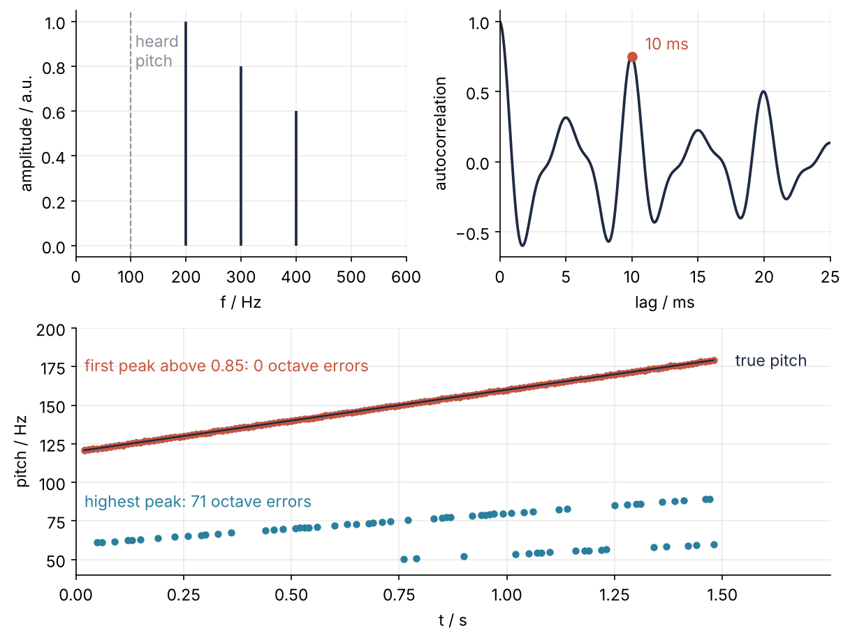
This is where we end up, drawn in Step 6: the missing fundamental on top, and below it the glide, where the rule "take the highest peak" puts 71 of 147 frames an octave or more too low and the rule "take the first strong peak" puts none there.
Setup
The cell fixes the pitch range searched, 50 to 400 Hz, and makes two sounds at 16 kHz. The first is the three tones, with amplitudes 1.0, 0.8, and 0.6 and random phases. The second stands in for a voice: a train of pulses, one every period \(1/f_0(t)\), like the puffs of air through the vocal folds, with \(f_0\) rising from 120 to 180 Hz over 1.5 s. Two resonances at 700 and 1,200 Hz, near those of the vowel in "father", give the sound its color; they are two-pole filters applied with lfilter, which Filtering with scipy.signal explains, and they shape the spectrum without moving the pulses.
Each pulse's height varies at random by about 10 %. In a voice this is called shimmer, and 10 % belongs to a pathological voice: in a healthy one it stays under about 4 %. I kept the rough voice on purpose, because it makes the test harder. White noise goes on top at a signal-to-noise ratio of 10 dB, and the true pitch is known only because we made the sound.
Nothing below depends on the sampling rate except through fs, so for your own recording read a WAV file with scipy.io.wavfile.read, which returns fs and the samples. They often come as 16-bit integers, and in stereo as two columns: data.astype(float), and for two channels .mean(axis=1), make the one float channel that the functions below expect.
import numpy as np
import matplotlib.pyplot as plt
from scipy.signal import correlate, correlation_lags, lfilter

plt.rcParams.update({
    "figure.figsize": (7, 3.6), "figure.dpi": 110,
    "axes.spines.top": False, "axes.spines.right": False,
    "axes.grid": True, "grid.alpha": 0.25,
    "font.size": 11, "lines.linewidth": 1.8,
})
INK, ACCENT, SECOND, MUTED = "#1f2a44", "#c8553d", "#2a7f9e", "#8a8f98"

fs = 16_000                          # samples per second
FRAME, HOP = 640, 160                # 40 ms frames, one every 10 ms
KMIN, KMAX = fs // 400, fs // 50     # lags of the pitch range, 400 Hz down to 50 Hz
rng = np.random.default_rng(275)

# three tones and no fundamental
t3 = np.arange(fs // 2) / fs
phases = rng.uniform(0, 2 * np.pi, 3)
x3 = sum(a * np.cos(2 * np.pi * f * t3 + p)
         for f, a, p in zip([200, 300, 400], [1.0, 0.8, 0.6], phases))

# a vowel-like glide from 120 to 180 Hz
DURATION = 1.5                       # s
t = np.arange(int(DURATION * fs)) / fs

def f0_true(t):
    return 120 + 60 * t / DURATION

cycles = np.cumsum(f0_true(t) / fs)                         # periods elapsed so far
pulses = np.flatnonzero(np.diff(np.floor(cycles))) + 1      # a pulse where a new period starts
source = np.zeros(t.size)
source[pulses] = 1 + 0.1 * rng.standard_normal(pulses.size)    # shimmer
voice = source
for fc, bw in [(700, 130), (1200, 150)]:                    # two resonances, in Hz
    rho = np.exp(-np.pi * bw / fs)
    voice = lfilter([1 - rho], [1, -2 * rho * np.cos(2 * np.pi * fc / fs), rho**2], voice)
voice = voice / voice.std()
voice = voice + 10 ** (-10 / 20) * rng.standard_normal(t.size)    # noise at 10 dB SNR

print(f"three tones: {x3.size} samples; glide: {voice.size} samples, {pulses.size} pulses, "
      f"{f0_true(0):.0f} to {f0_true(DURATION):.0f} Hz")
three tones: 8000 samples; glide: 24000 samples, 224 pulses, 120 to 180 Hz
Step 1: Look at the spectrum, and see it miss the pitch
Take the first 40 ms of the three tones and compute the amplitude spectrum as in the prerequisite. With 640 samples the bins are 25 Hz apart, so all three tones sit exactly on bins and need no window.
N = FRAME
frame3 = x3[:N]
freqs = np.fft.rfftfreq(N, 1 / fs)
amp = 2 * np.abs(np.fft.rfft(frame3)) / N

for i in np.argsort(amp)[::-1][:3]:
    print(f"{freqs[i]:4.0f} Hz   amplitude {amp[i]:.2f}")
print(f"{100:4d} Hz   amplitude {amp[freqs == 100][0]:.2f}")
 200 Hz   amplitude 1.00
 300 Hz   amplitude 0.80
 400 Hz   amplitude 0.60
 100 Hz   amplitude 0.00
The spectrum has exactly what we put in, and its highest peak is 200 Hz. Now look at the waveform:
Show code
fig, ax = plt.subplots(figsize=(7, 3))
ms = 1000 * t3
ax.plot(ms[ms <= 30], x3[ms <= 30], color=INK)
for m in [10, 20]:
    ax.axvline(m, color=MUTED, ls="--", lw=1)
ax.set(xlabel="t / ms", ylabel="amplitude / a.u.", xlim=(0, 30))
plt.show()
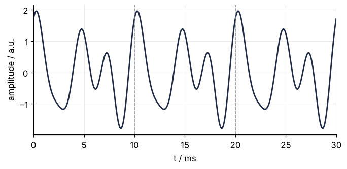
No 10 ms sine is in it, yet the same shape comes back every 10 ms. That repetition is what the ear hears as the pitch. In a notebook, IPython.display.Audio(x3, rate=fs) lets you hear it too.
Step 2: Autocorrelate a frame with scipy.signal.correlate
The autocorrelation compares a signal with a copy of itself shifted by \(k\) samples: multiply the two sample by sample and add up the products. Where the copy lines up with the original, every product is positive and the sum is large. For a frame \(x_0, \dots, x_{N-1}\),
correlate computes this for every shift, and correlation_lags says which shift each value belongs to. At lag \(k\) the sum has only \(N - k\) products, so long lags come out small even for a signal that repeats perfectly. The cell therefore divides it two ways: by the frame length \(N\), which statisticians call "biased", because as an estimate for an endless signal it is too small at long lags, and by the number of products \(N - k\), called "unbiased". Both are scaled to 1 at lag 0 and compared at the period, 10 ms, and at twice the period:
r3 = correlate(frame3, frame3, mode="full")
lags = correlation_lags(N, N, mode="full")
print(f"{r3.size} values, lags {lags[0]} to {lags[-1]}")

r3, lags = r3[lags >= 0], lags[lags >= 0]
r_biased = r3 / r3[0]                       # r/N, scaled to 1 at lag 0
r_unbiased = r3 / (N - lags)                # divided by the number of products
r_unbiased /= r_unbiased[0]
for k in [0, 160, 320]:
    print(f"lag {k:3d} = {1000 * k / fs:4.1f} ms   r/N {r_biased[k]:.2f}   r/(N - k) {r_unbiased[k]:.2f}")

k_peak = KMIN + np.argmax(r_biased[KMIN:KMAX + 1])
print(f"highest peak in range: lag {k_peak} = {1000 * k_peak / fs:.1f} ms -> {fs / k_peak:.1f} Hz")
1279 values, lags -639 to 639
lag   0 =  0.0 ms   r/N 1.00   r/(N - k) 1.00
lag 160 = 10.0 ms   r/N 0.75   r/(N - k) 1.00
lag 320 = 20.0 ms   r/N 0.50   r/(N - k) 1.00
highest peak in range: lag 160 = 10.0 ms -> 100.0 Hz
The negative lags are dropped because \(r(-k) = r(k)\): shifting left or right by \(k\) pairs the same samples. Dividing by \(r(0)\) makes the value at lag 0 equal to 1.
Show code
fig, ax = plt.subplots(figsize=(7, 3))
lag_ms = 1000 * lags / fs
keep = lag_ms <= 20
ax.plot(lag_ms[keep], r_biased[keep], color=INK)
ax.axvline(10, color=MUTED, ls="--", lw=1)
ax.plot(10, r_biased[160], "o", color=ACCENT, ms=6)
ax.annotate("10 ms = 100 Hz", (10, r_biased[160]), xytext=(11, 0.85), color=ACCENT)
ax.set(xlabel="lag / ms", ylabel="autocorrelation", xlim=(0, 20))
plt.show()
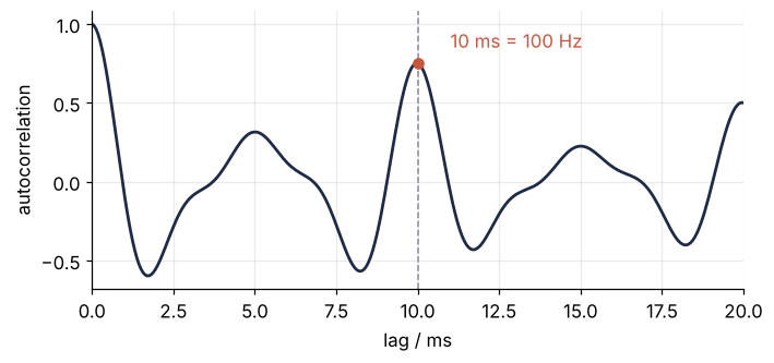
The highest peak in the search range sits at lag 160, 10 ms, which is 100 Hz: the heard pitch. The biased peak is 0.75, not 1, and only 0.50 at 20 ms, because at lag 160 a quarter of the frame has slid off the end. The unbiased one puts both at 1.00, so heights compare across lags, which is why Steps 4 to 6 use it; Autocorrelation takes the two apart. It no longer prefers 10 ms over 20 ms, and Step 5 shows what that costs.
Step 3: Compute the same with the FFT
The autocorrelation is the inverse Fourier transform of the power spectrum \(|X|^2\), a result known as the Wiener-Khinchin theorem. There is one catch. The FFT treats the frame as one period of an endless repetition, so a copy shifted by \(k\) samples comes back in at the other end, and products of the frame's end with its start enter every sum. Padding the frame with \(N\) zeros makes the part that wraps around zero. This is a different reason for padding than in the prerequisite, where padding only drew the peaks more smoothly.
X = np.fft.rfft(frame3, n=2 * N)
r_fft = np.fft.irfft(np.abs(X) ** 2, n=2 * N)[:N]
print(f"largest difference from correlate: {np.max(np.abs(r_fft - r3)) / r3[0]:.1e} of r(0)")
largest difference from correlate: 3.6e-16 of r(0)
The two agree to rounding. The direct sum costs about \(N^2\) multiplications, the FFT about \(N \log N\). correlate with its default method="auto" picks the FFT itself when the inputs are long, and method="fft" forces it.
Step 4: Find the period peak and refine it with a parabola
Now a frame of the glide, the one centered at 0.62 s. The function below computes the unbiased autocorrelation, finds the local maxima in the search range, and takes the highest. A lag is a whole number of samples, so its pitch can be off by up to half a sample. The fix is to fit a parabola through the peak sample and its two neighbors, with heights \(r_-\), \(r_0\), \(r_+\), and take its vertex. The vertex lies
samples from the middle one. The keyword threshold is for Step 6, and its line rests on one NumPy idiom: np.argmax of a boolean array returns the index of the first True. So the line picks the first local maximum at least threshold times as tall as the highest, and at 1.0 only the highest qualifies.
def autocorr(frame, unbiased=True):
    N = len(frame)
    r = correlate(frame, frame, mode="full")[N - 1:]       # lags 0 to N - 1
    if unbiased:
        r = r / (N - np.arange(N))
    return r / r[0]

def period(frame, threshold=1.0, unbiased=True):
    """The period in samples, to a fraction of a sample."""
    r = autocorr(frame, unbiased)
    k = np.arange(KMIN, min(KMAX, len(frame) - 2) + 1)
    k = k[(r[k] > r[k - 1]) & (r[k] >= r[k + 1])]          # local maxima
    k = k[np.argmax(r[k] >= threshold * r[k].max())]       # the first one tall enough
    r_m, r_0, r_p = r[k - 1], r[k], r[k + 1]
    return k + 0.5 * (r_m - r_p) / (r_m - 2 * r_0 + r_p)

start = 60 * HOP
frame = voice[start:start + FRAME]
f_c = f0_true((start + FRAME / 2) / fs)
r = autocorr(frame)
k_int = KMIN + np.argmax(r[KMIN:KMAX + 1])
T = period(frame)
print(f"integer lag {k_int:7.2f} samples -> {fs / k_int:6.2f} Hz")
print(f"parabola    {T:7.2f} samples -> {fs / T:6.2f} Hz")
print(f"truth       {fs / f_c:7.2f} samples -> {f_c:6.2f} Hz")
integer lag  111.00 samples -> 144.14 Hz
parabola     110.51 samples -> 144.78 Hz
truth        110.50 samples -> 144.80 Hz
Show code
ks = np.arange(k_int - 6, k_int + 7)
r_m, r_0, r_p = r[k_int - 1], r[k_int], r[k_int + 1]
a, b = (r_m + r_p) / 2 - r_0, (r_p - r_m) / 2                 # r = r_0 + b x + a x^2
x = np.linspace(-1.5, 1.5, 100)
fig, ax = plt.subplots(figsize=(7, 3))
ax.plot(ks, r[ks], "o", color=INK, ms=6)
ax.plot(k_int + x, r_0 + b * x + a * x**2, color=ACCENT)
ax.plot(T, r_0 - b**2 / (4 * a), "D", color=ACCENT, ms=6)
ax.axvline(fs / f_c, color=MUTED, ls="--", lw=1)
ax.text(T - 0.2, 0.89, f"vertex {T:.2f}", color=ACCENT, ha="right")
ax.text(fs / f_c - 0.25, -0.25, f"true lag {fs / f_c:.2f}", color=MUTED, ha="right")
ax.set(xlabel="lag / samples", ylabel="autocorrelation", ylim=(-0.35, 1.0))
plt.show()
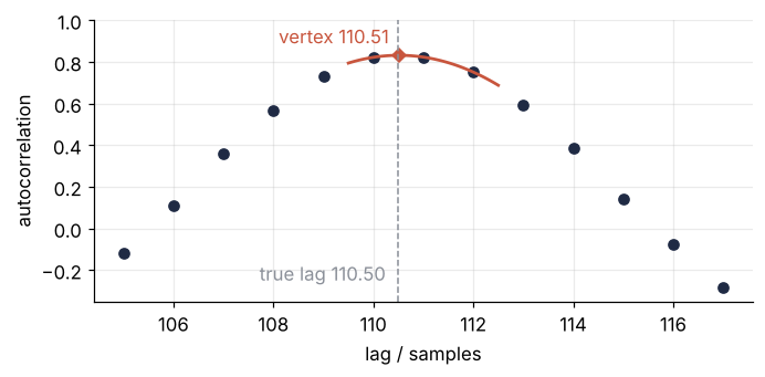
The integer lag is 111 samples, 144.14 Hz, which is 0.66 Hz too low. The parabola puts the vertex at 110.51 samples against a true 110.50, and the pitch within 0.02 Hz. In the zoom the vertex lands between two samples, on the dashed line of the true lag. The local maxima come from comparing each sample with both neighbors, one line of NumPy; for peaks that need a prominence condition, Find peaks with scipy.signal.find_peaks is the tool.
Step 5: Track the pitch frame by frame, and meet octave errors
Run period on every 40 ms frame, one every 10 ms, and compare with the true pitch at the frame's center. Call an estimate \(f\) an octave error when it is closer to half or double the true pitch \(f_0\) than to \(f_0\) itself, that is, when \(|\log_2(f/f_0)| > 1/2\); anything further off counts too.
starts = np.arange(0, voice.size - FRAME + 1, HOP)
f_true = f0_true((starts + FRAME / 2) / fs)

def track(**kw):
    return np.array([fs / period(voice[s:s + FRAME], **kw) for s in starts])

f_highest = track()
octave = np.abs(np.log2(f_highest / f_true)) > 0.5
share = np.round(f_true / f_highest)
print(f"{octave.sum()} of {starts.size} frames off by an octave or more: "
      f"{np.sum(share == 2)} at half the pitch, {np.sum(share == 3)} at a third")
print(f"median error of the others: {np.median(np.abs(f_highest - f_true)[~octave]):.2f} Hz")
71 of 147 frames off by an octave or more: 53 at half the pitch, 18 at a third
median error of the others: 0.09 Hz
Show code
t_frames = (starts + FRAME / 2) / fs
fig, ax = plt.subplots(figsize=(7, 3.4))
ax.plot(t_frames, f_true, color=INK)
for d, name in [(2, "half"), (3, "a third")]:
    ax.plot(t_frames, f_true / d, color=MUTED, ls="--", lw=1)
    ax.text(1.53, f_true[-1] / d, name, color=MUTED, va="center")
ax.plot(t_frames, f_highest, "o", color=SECOND, ms=4)
ax.text(1.53, f_true[-1], "true pitch", color=INK, va="center")
ax.set(xlabel="t / s", ylabel="pitch / Hz", xlim=(0, 1.8), ylim=(30, 200), xticks=np.arange(0, 1.6, 0.25))
plt.show()
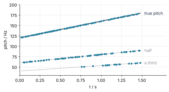
In 71 of 147 frames the estimate is too low, 53 at half the pitch and 18 at a third, while the median error of the rest is 0.09 Hz. The unbiased autocorrelation of a periodic sound has equally tall peaks at the period \(T\) and at \(2T\) and \(3T\), as the 1.00 at both 10 and 20 ms showed in Step 2. In the glide the noise and shimmer from Setup make them differ by a few hundredths, and which one is highest is a coin toss.
Step 6: Take the first strong peak, and count again
Instead of the highest peak, take the first one, at the shortest lag, whose height is at least \(\theta\) times the highest, with \(\theta = 0.85\); in period that is the threshold line. Here is the frame at 0.68 s, which the highest-peak rule got wrong:
Show code
start = 66 * HOP
frame = voice[start:start + FRAME]
r = autocorr(frame)
k = np.arange(KMIN, KMAX + 1)
k = k[(r[k] > r[k - 1]) & (r[k] >= r[k + 1])]
k_T, k_2T = k[np.argmax(r[k] >= 0.85 * r[k].max())], k[np.argmax(r[k])]
print(f"true period {fs / f0_true((start + FRAME / 2) / fs):.1f} samples; "
      f"peak at lag {k_T}: {r[k_T]:.3f}, peak at lag {k_2T}: {r[k_2T]:.3f}")

fig, ax = plt.subplots(figsize=(7, 3))
ax.plot(np.arange(KMAX + 1), r[:KMAX + 1], color=INK)
ax.axhline(0.85 * r[k_2T], color=MUTED, ls="--", lw=1)
ax.plot(k_T, r[k_T], "o", color=ACCENT, ms=7)
ax.plot(k_2T, r[k_2T], "o", color=SECOND, ms=12, mfc="none", mew=1.5)
ax.text(k_T + 6, r[k_T] + 0.05, f"lag {k_T}", color=ACCENT)
ax.text(k_2T + 6, r[k_2T] + 0.05, f"lag {k_2T}", color=SECOND)
ax.text(KMAX - 4, 0.85 * r[k_2T] - 0.04, "θ × highest", color=MUTED, ha="right", va="top")
ax.set(xlabel="lag / samples", ylabel="autocorrelation", xlim=(0, KMAX), ylim=(-0.8, 1.15))
plt.show()
true period 108.7 samples; peak at lag 109: 0.902, peak at lag 218: 0.919
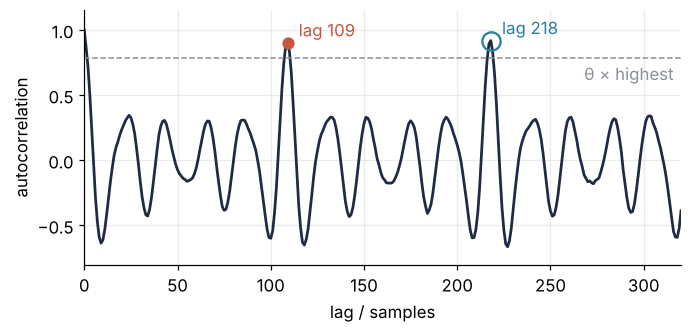
The period peak at lag 109 reaches 0.902; the one at lag 218 reaches 0.919 and won by 0.017. Both clear the dashed line, and the first above it is the period. Now the whole glide, for six values of \(\theta\) and for the biased autocorrelation:
print("   θ    octave low   too high")
for theta in [1.0, 0.95, 0.85, 0.7, 0.5, 0.3]:
    ratio = np.log2(track(threshold=theta) / f_true)
    print(f"{theta:4.2f}   {np.sum(ratio < -0.5):8d}   {np.sum(ratio > 0.5):8d}")

f_biased = track(unbiased=False)
print(f"biased, highest peak: {np.sum(np.abs(np.log2(f_biased / f_true)) > 0.5)} octave errors")
for f in [f_true[66], 400]:
    T = fs / f
    print(f"{f:5.1f} Hz: the biased rule acts like θ = {(FRAME - 2 * T) / (FRAME - T):.2f}")
   θ    octave low   too high
1.00         71          0
0.95         11          0
0.85          0          0
0.70          0          0
0.50          0          0
0.30          0         58
biased, highest peak: 0 octave errors
147.2 Hz: the biased rule acts like θ = 0.80
400.0 Hz: the biased rule acts like θ = 0.93
At \(\theta = 1\), 71 frames are too low, at 0.95 still 11, from 0.85 down to 0.5 none. At 0.3, 58 frames come out too high: the resonances leave small peaks at a fraction of the period, which a low \(\theta\) accepts.
The biased rule makes no octave error here, and not by accident. Dividing by \(N\) shrinks the peak at lag \(k\) by \((N-k)/N\), so comparing the peaks at \(2T\) and \(T\) amounts to a threshold
which is 0.80 at the 147.2 Hz of the frame above but 0.93 at 400 Hz, nearly as strict as the 0.95 that left 11 errors. It moves with the pitch and the frame length. On your own data, use the unbiased autocorrelation with an explicit \(\theta\), the same at every pitch. Start at 0.85, lower it if the track drops by octaves, raise it if it jumps up, and check it on a stretch whose pitch you know.
f_first = track(threshold=0.85)
n_first = np.sum(np.abs(np.log2(f_first / f_true)) > 0.5)
print(f"first peak above 0.85: {n_first} octave errors, "
      f"median error {np.median(np.abs(f_first - f_true)):.2f} Hz")
first peak above 0.85: 0 octave errors, median error 0.09 Hz
Show code
fig, axs = plt.subplot_mosaic([["spec", "acf"], ["track", "track"]],
                              figsize=(8, 6), layout="constrained")
ax = axs["spec"]
ax.vlines(freqs, 0, amp, color=INK)
ax.axvline(100, color=MUTED, ls="--", lw=1)
ax.text(108, 0.8, "heard\npitch", color=MUTED)
ax.set(xlabel="f / Hz", ylabel="amplitude / a.u.", xlim=(0, 600))
ax = axs["acf"]
keep = lag_ms <= 25
ax.plot(lag_ms[keep], r_biased[keep], color=INK)
ax.plot(10, r_biased[160], "o", color=ACCENT, ms=6)
ax.text(11, 0.8, "10 ms", color=ACCENT)
ax.set(xlabel="lag / ms", ylabel="autocorrelation", xlim=(0, 25))
ax = axs["track"]
ax.plot(t_frames, f_highest, "o", color=SECOND, ms=4)
ax.plot(t_frames, f_first, "o", color=ACCENT, ms=4)
ax.plot(t_frames, f_true, color=INK, lw=1.2)                            # on top of the dots
ax.text(1.53, f_true[-1], "true pitch", color=INK, va="center")
ax.text(0.02, 172, f"first peak above 0.85: {n_first} octave errors", color=ACCENT)
ax.text(0.02, 84, f"highest peak: {octave.sum()} octave errors", color=SECOND)
ax.set(xlabel="t / s", ylabel="pitch / Hz", xlim=(0, 1.75), ylim=(40, 200), xticks=np.arange(0, 1.6, 0.25))
plt.show()
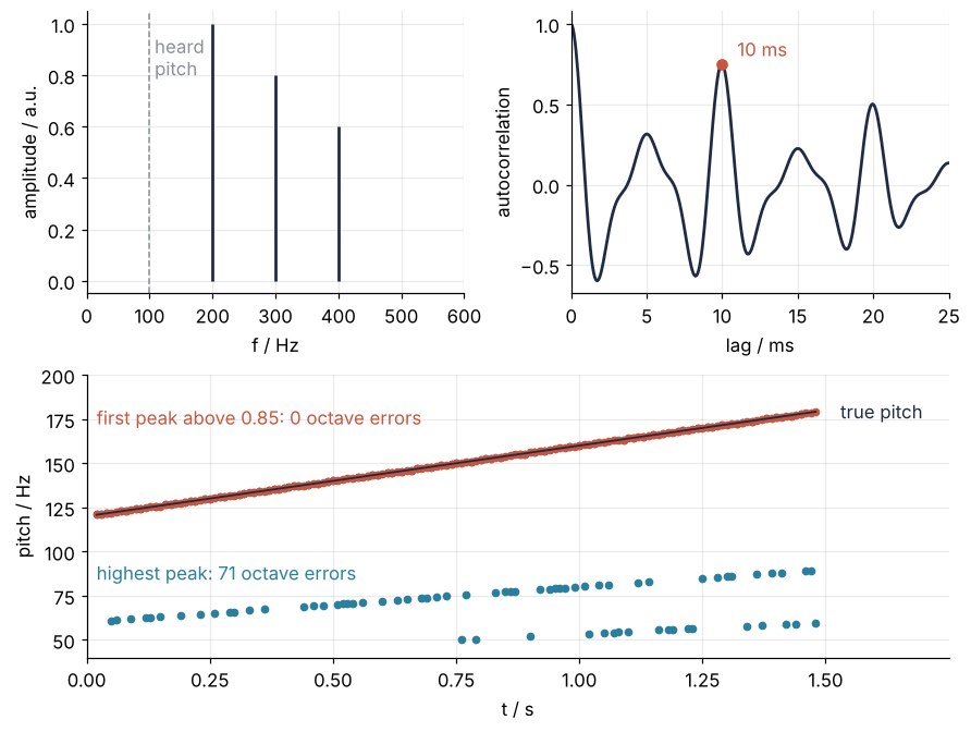
With \(\theta = 0.85\) no frame is off by an octave, and the median error is 0.09 Hz, against the 0.66 Hz by which the integer lag missed in Step 4.
Pitfalls
Lags too long for the frame. Shorten the frame to 20 ms to follow a pitch that changes fast, keep the search down to 50 Hz, and the track falls apart even with \(\theta = 0.85\). Plot the unbiased autocorrelation of a 40 ms frame out to its end, and the last stretch looks like a strong signal, higher than at lag 0, where a signal matches itself perfectly:
SHORT = 320                                                 # 20 ms
starts_20 = np.arange(0, voice.size - SHORT + 1, HOP)
f_20 = np.array([fs / period(voice[s:s + SHORT], 0.85) for s in starts_20])
bad = np.abs(np.log2(f_20 / f0_true((starts_20 + SHORT / 2) / fs))) > 0.5
print(f"20 ms frames, θ = 0.85: {bad.sum()} of {starts_20.size} off by an octave or more")
tail = np.array([autocorr(voice[s:s + FRAME])[500:].max() for s in starts])
print(f"40 ms frames beyond lag 500: largest value {tail.max():.2f}, above 1 in {100 * np.mean(tail > 1):.0f} % of frames")
20 ms frames, θ = 0.85: 58 of 149 off by an octave or more
40 ms frames beyond lag 500: largest value 3.62, above 1 in 48 % of frames
The short frames put 58 of 149 estimates off by an octave, against none of the 40 ms frames, and the long frames reach 3.62 beyond lag 500. Both symptoms have one cause: at lag 600 the sum has 40 products, at lag 630 only ten, and dividing by so few turns noise into peaks. In a 20 ms frame the search reaches lag 318, where two products remain, so the highest peak against which \(\theta\) is measured is noise and the period peak falls below the line. Read the unbiased autocorrelation only out to half the frame, which is what KMAX = \(N/2\) does here: the frame must hold two of the longest periods searched, 40 ms for 50 Hz. If it has to be short, raise the lowest pitch searched instead.
A pitch in every frame. period returns a number for anything, also for a pause or a breath, which a real recording has and the synthetic glide does not. Feed it the noise of Setup alone:
def chosen_height(frame):
    return autocorr(frame)[round(period(frame, 0.85))]

hiss = 10 ** (-10 / 20) * rng.standard_normal(FRAME)        # the noise of Setup, no voice
lowest = min(chosen_height(voice[s:s + FRAME]) for s in starts)
print(f"noise alone: {fs / period(hiss, 0.85):.0f} Hz from a peak of {chosen_height(hiss):.2f}; "
      f"lowest chosen peak in the glide: {lowest:.2f}")
noise alone: 110 Hz from a peak of 0.11; lowest chosen peak in the glide: 0.79
The noise gets a pitch of 110 Hz, inside the range of the glide, from a peak of 0.11, while no frame of the glide chose a peak below 0.79. Keep the height of the chosen peak with every estimate, and call a frame unvoiced when it falls under a limit between the two, checked on a stretch of your recording you know is silent. A frame of digital silence has \(r(0) = 0\), and autocorr divides by it: skip such frames before the call.
The FFT without padding. irfft(abs(rfft(frame))**2) looks like an autocorrelation and agrees with correlate at lag 0, but nowhere else:
r_wrapped = np.fft.irfft(np.abs(np.fft.rfft(frame3)) ** 2, n=N)
print(f"largest difference from correlate: {np.max(np.abs(r_wrapped - r3)) / r3[0]:.2f} of r(0)")
largest difference from correlate: 0.99 of r(0)
The difference reaches 0.99 of \(r(0)\), against \(3.6 \times 10^{-16}\) with padding in Step 3. The cause is the wrap-around of Step 3: without padding, every sum but the one at lag 0 also contains the products of the frame's end with its start, so lag \(k\) returns \(r(k) + r(N - k)\). Pad to n=2 * N or more; scipy.fft.next_fast_len(2 * N - 1) gives a length at which the FFT is fast.
Variations
- The YIN difference function. Replace the autocorrelation by the squared difference \(d(k) = \sum_n (x_n - x_{n+k})^2\), divide each \(d(k)\) by its mean over lags 1 to \(k\), and take the first dip below 0.1. It is the threshold of Step 6, turned upside down (de Cheveigné and Kawahara 2002).
- Heart rate from a pulse signal. Run
periodon the pulse signal of Find peaks with scipy.signal.find_peaks, sampled at 100 Hz, with 5 s frames and a search range of 40 to 180 beats per minute, lags 33 to 150. The rate comes out without picking a single beat. - Vibration period from an accelerometer. A machine turning at 1,500 rpm shakes once per turn, every 40 ms. Set
fsto the logger's rate and the search range around the speeds the machine runs at. - Birdsong. Pitches of 2 to 8 kHz need
fs= 44.1 kHz, which puts the periods at lags of 5 to 22 samples. A 2 ms frame of 88 samples still holds the longest period four times.
Cheat sheet
r = correlate(x, x, mode="full")[N - 1:]           # lags 0 to N - 1; FFT: irfft(abs(rfft(x, 2*N))**2)[:N]
r = r / (N - np.arange(N)); r /= r[0]              # unbiased: 1 at every period of a periodic signal
kmin, kmax = int(fs / f_max), int(fs / f_min)      # pitch range in lags; kmax <= N // 2
k = np.arange(kmin, kmax + 1)
k = k[(r[k] > r[k - 1]) & (r[k] >= r[k + 1])]      # local maxima
k = k[np.argmax(r[k] >= 0.85 * r[k].max())]        # the first peak above θ × highest, not the highest
rm, r0, rp = r[k - 1], r[k], r[k + 1]
T = k + 0.5 * (rm - rp) / (rm - 2 * r0 + rp)       # parabola vertex, in samples
f0 = fs / T                                        # pitch in Hz
Further reading
- The SciPy reference for
scipy.signal.correlateandscipy.signal.correlation_lags, with themethodkeyword that chooses between the direct sum and the FFT. - P. Boersma, "Accurate short-term analysis of the fundamental frequency and the harmonics-to-noise ratio of a sampled sound", Proceedings of the Institute of Phonetic Sciences 17 (1993) 97, the autocorrelation method behind the speech program Praat, with a careful treatment of the normalization.
- A. de Cheveigné and H. Kawahara, "YIN, a fundamental frequency estimator for speech and music", Journal of the Acoustical Society of America 111 (2002) 1917.
- L. R. Rabiner and R. W. Schafer, Theory and Applications of Digital Speech Processing (Pearson, 2011), for pitch detection in speech.
- Related tutorials on this site: The Fourier transform: asking a signal how much of each frequency it contains, Autocorrelation: how many independent hours a year of wind power holds, Find peaks with scipy.signal.find_peaks: heartbeats in a noisy pulse signal, Dynamic light scattering: nanoparticle size from the flicker of laser light, Find where sampled data cross a level: a peak's full width at half maximum, and Plucked string harmonics: why a pluck at a third has no third harmonic. Planned: The same pitch tracker in Julia.
- Download the notebook. It was executed with the library versions in the header.